Gridded modelling of GB wind generation and electricity demand to 2035:
Disaggregation of National Grid annual scenarios
Ed Sharp:
ed.sharp@ucl.ac.uk | www.esenergyvis.wordpress.com | @steadier_eddy
Context
- Scenarios are designed to counteract some of the uncertainty in projecting change to the energy system.
- Due to this uncertainty, however, it is unrealistic to perform this scenario modelling at a lower resolution than national, annual
- Therefore uncertainty remains on the implications of these scenarios, particularly when aspects of supply and demand which fluctuate at small resolutions such as those which are driven by weather are introduced/increased.
- The view of my research is that if scenarios are predetermined it is possible to reduce this uncertainty through disaggregated modelling.
- Also very importantly that demand should be modelled, to allow the consideration of new demand, not just growth of existing demands.
Why model on a grid?
Research hypothesis
“National annual resolution scenario modelling can be complemented through spatiotemporally disaggregated modelling which captures the inherent variability of wind generation and weather driven electricity demand; furthermore, disaggregation of scenarios can be achieved using existing methods and data.”
Gridded Approach
- Disaggregation can be carried out using any spatial units, though practically the choice is between census geographies (at any resolution) and grid.
- Here the grid is used for a number of reasons
- Data availability (especially weather – NCEP CFSR)
- •Flexibility in programming, arrays vs. databases
- Homogeneity
- Time: Census geographies change over time
- Space: especially over offshore areas
- The model grid
- 0.5 degree lat/lon grid
- >200 onshore grid squares
Why model on a grid?

Method - Wind Generation
Wind generation: estimating hourly generation using CFSR
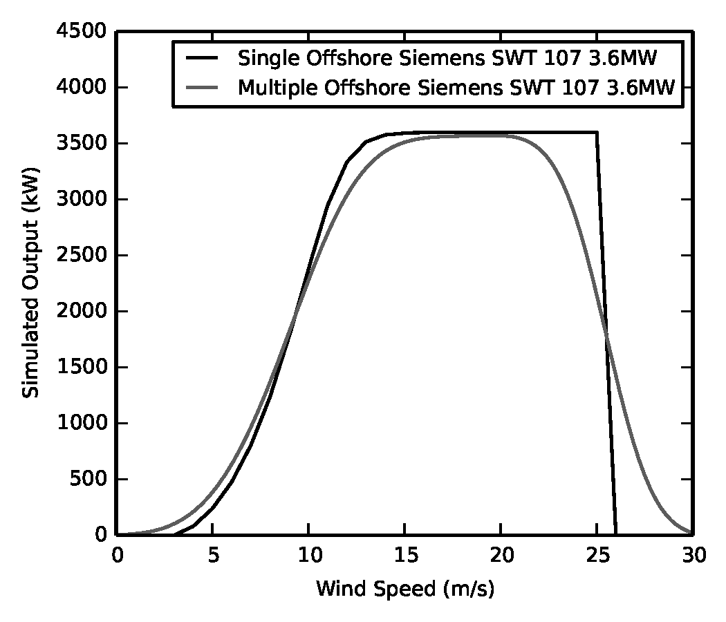
- Simple method
- Archetype curves (onshore/offshore)
- Temporally and spatially consistent wind speed height correction
- Could be improved but evaluation performed
- Grid point wind speed data not interpolated
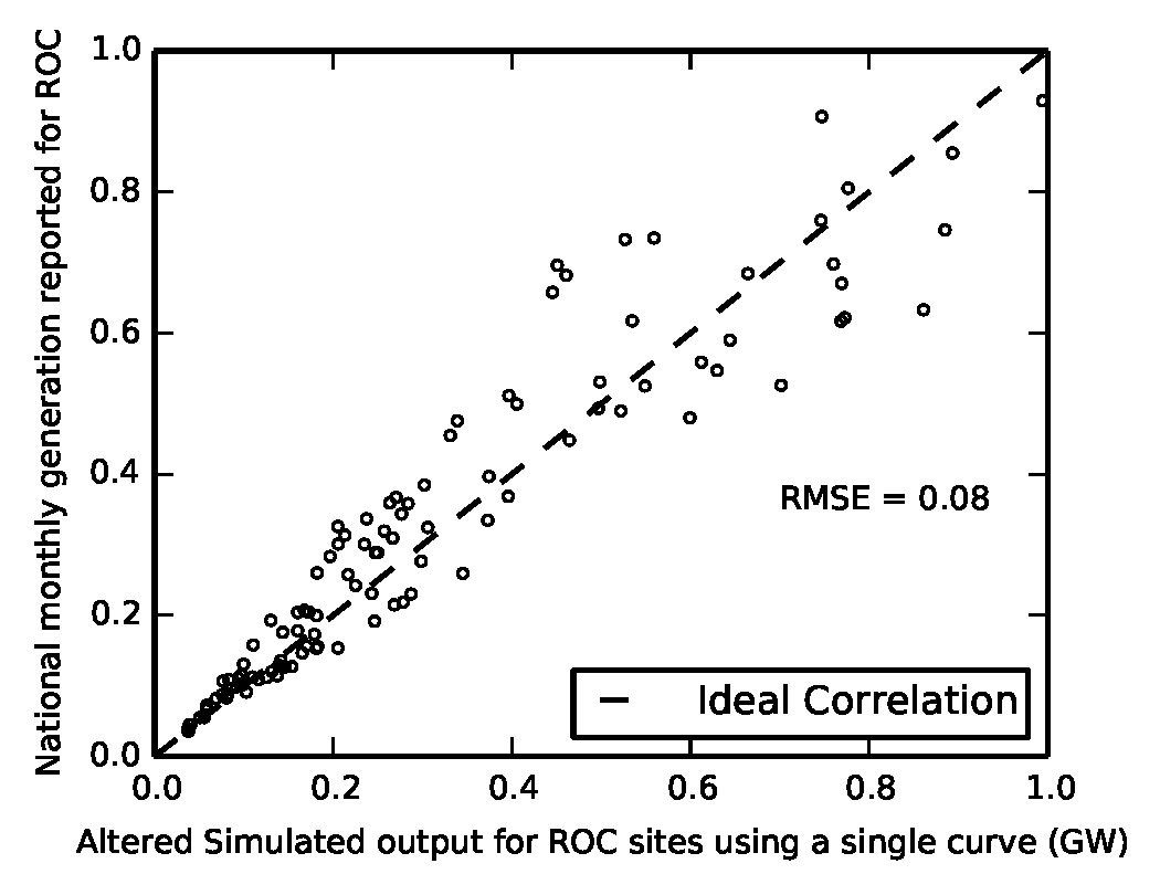
- Reasonable accuracy achieved
- Projections do not rely on totally accurate method, due to uncertainty over future capacity
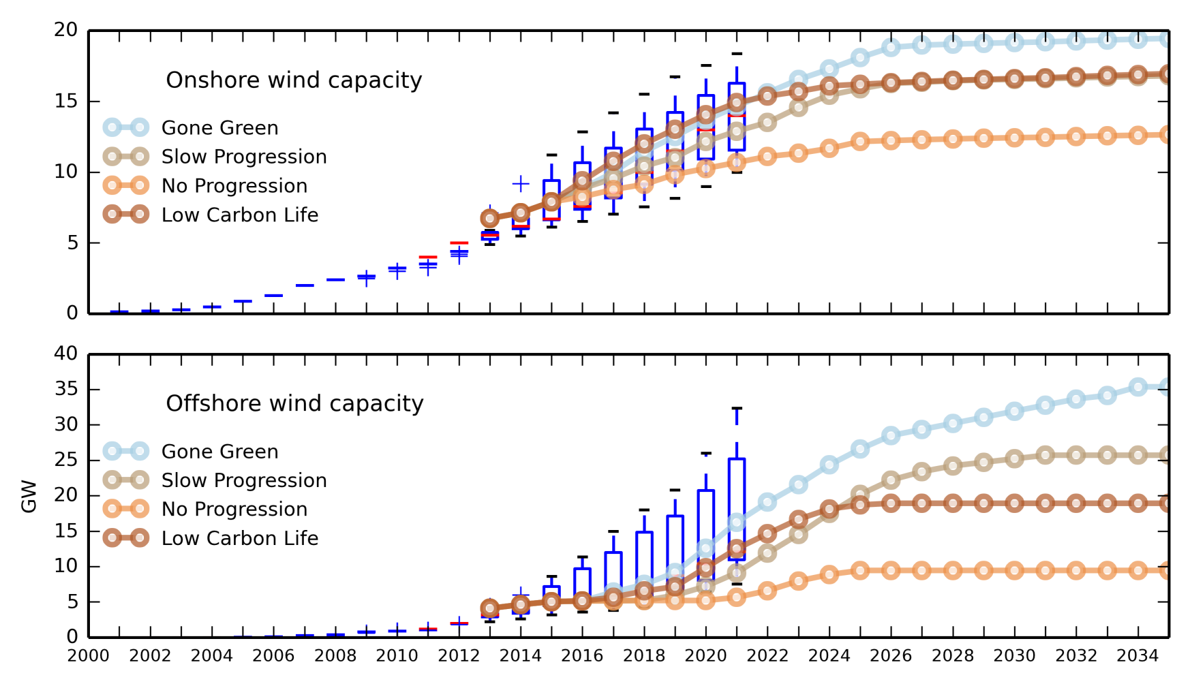
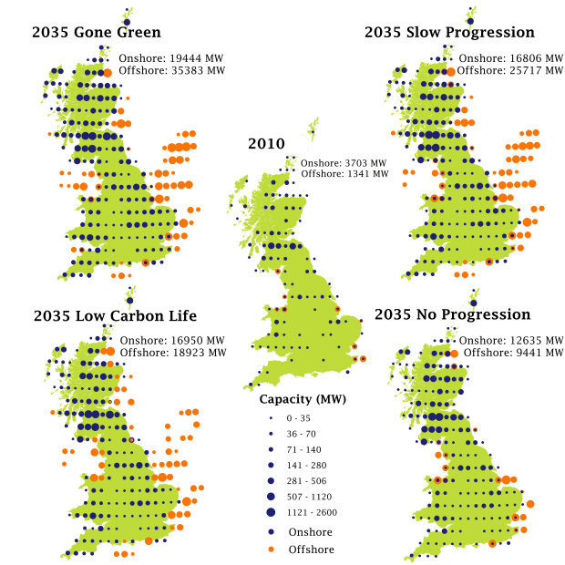
Wind generation: estimating hourly generation from different capacities
- Site specific approach would have yielded more accurate results
- The gridded approach however facilitates disaggregation of scenarios, without the need to select exact farm locations
- How can National Grid’s scenarios be redistributed to the model grid?
Wind generation: estimating hourly generation from different capacities
Step 1: Eliminate unsuitable areas
- Constraints on development identified from the literature
- Particularly resource estimation studies
- Spatial data collated
- Tested against operational capacity
- Small number of farms within these zones
- 31% of GB removed from consideration
- In reality there are further restrictions e.g. from social acceptability
- However very low likelihood areas are removed
- This analysis removes sites above 600 m.

Wind generation: estimating hourly generation from different capacities
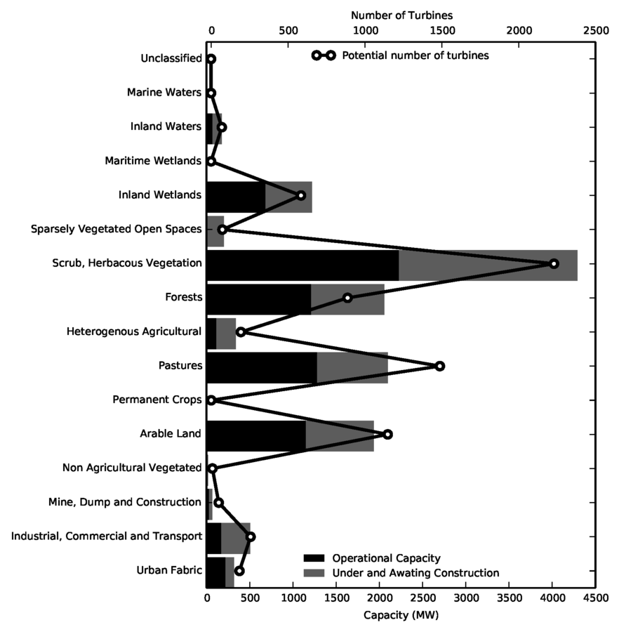
Step 2: Identify suitable land uses
- Using locations of existing wind farms and land use mapping
- Clearly four commonly used land types
- These take precedence in subsequent allocation
Step 3: Identify high wind sites
- Characterising wind speed from CFSR by grid square in long term >30 years shows all GB grid squares suitable
Wind generation: estimating hourly generation from different capacities
Step 4: Allocate capacity to grid
- Fill available land
- Prioritise high wind, land uses, spatial diversity
- Generous assumptions made on turbine spacing (using archetypes)
- Offshore use development zones
- Ample space for all scenarios
Wind generation: Animation
Method –
Estimating hourly electricity demand
Electricity demand: overview of method
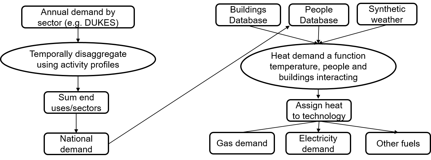
Top Down
Bottom Up
- Weather independent, building independent, e.g. cooking
- Advantages: simplicity, available data
- Disadvantages: difficult to model changes in the way energy is used
- Dependent on weather and building fabric
- Advantages: model changes in the way energy is used
- Disadvantages: more complex data needed
Electricity demand: people in SpDEAM
-
Domestic demands must be disaggregated to the grid so that wasted heat can be included in the heat demand equation
- Gridded population data used (Gridded Population of the World)
-
Assumed that people use the same amount of energy
- Could be changed
- Adapted to % of pop in each grid square, this remains static in scenario modelling, absolute population changes
- The model structure does however provide the ability to model migration etc.
- Heat from people calculated from pop database
- Assuming even distribution across building types (see buildings in next slide)
Electricity demand: buildings in SpDEAM
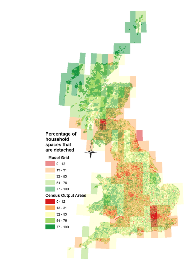
- Dwellings heated to desired internal temperature (only heating) from external T (CFSR)
-
Heat loss dependent on dwelling type and floor area
- Calculated using census data
- Scenarios increase housing stock and change heat loss coefficients (including the effect of demolitions)
- Solar gains assuming glazed area using CFSR data
-
Incidental gains calculated from redistributed top down demands
- Evenly distributed amongst dwelling types (could be altered)
Electricity demand: heating technologies in SpDEAM
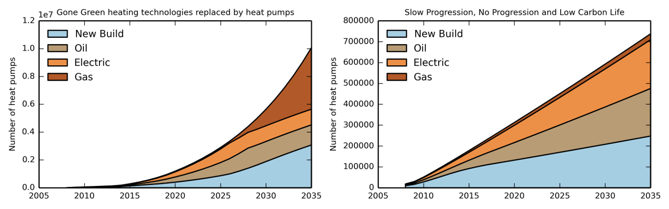
-
Heat demand Assigned to heating technologies based on census central heating data (E and W only, Scotland needed assumptions)
- Uniformly distributed across dwelling types
- These are adapted in scenario modelling to represent the introduction of heat pumps
- Relationship between COP and external T derived from field trials
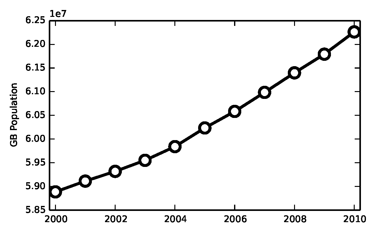
Electricity demand: calibration and evaluation of SpDEAM
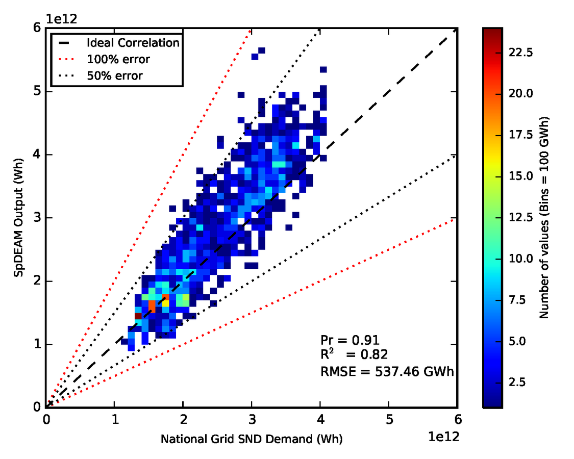
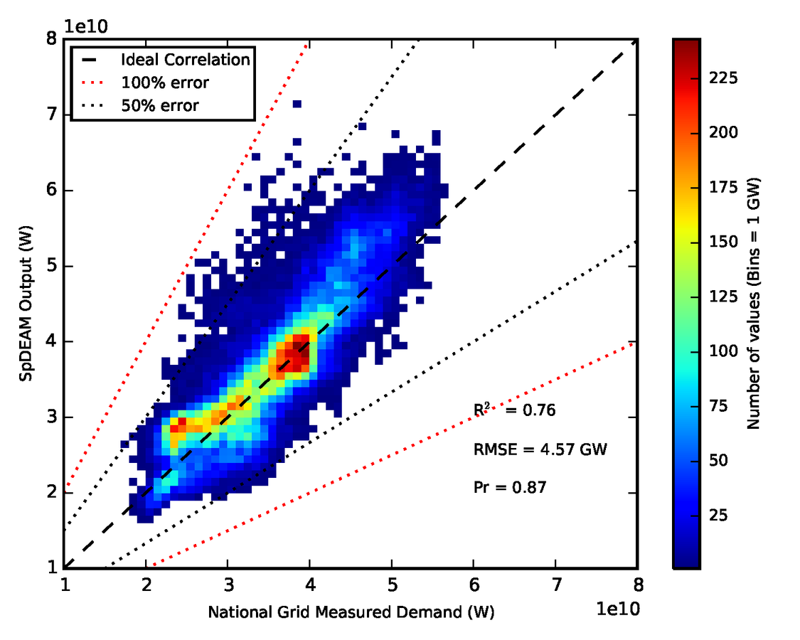
- Calibrated from 2000 – 2010
- Evaluated 2010 – 2014
- Remarkably accurate given the challenge of modelling the entire GB electricity system with limited data and necessary simplification and grouping of demands
All electricity demand - hourly
All gas demand - daily
Analysis - residual electricity demand
Residual Electricity Demand:
Animation
- November 2033
- Evidence of weather fronts
- Though often wind generation is variable onshore
- Periods of negative residual demand
- Requires high on and offshore generation
- Demand centred on small number of grid squares
- Low or negative residual demand is persistent across large number of grid squares
- Therefore transmission is key
- Low wind occurs on and offshore but both are rare
Publications:
- Thesis available at: https://goo.gl/ETYWiO
- Blog: www.esenergyvis.wordpress.com
- Sharp, E. Dodds, P. Barrett, M. and Spataru, C. Evaluating the accuracy of CFSR reanalysis hourly wind speed forecasts for the UK, using in situ measurements and geographical information. Renewable Energy, 77, 527-538. 2015. https://goo.gl/gJrcR1
- Sharp, E. Spatiotemporal Disaggregation of GB Scenarios Depicting Increased Wind Capacity and Electrified Heat Demand in Dwellings. 38th IAEE International Conference, Antalya, Turkey, 2015.
- Sharp, E. Spataru, C. Barrett, M. and Dodds, P. Incorporating building specific heat loss and associated energy demand into electricity demand models for Great Britain. Building Simulation and Optimisation UCL, London, UK, 2014.
Contact etc.:
Email: ed.sharp@ucl.ac.uk
Linkedin: ed.sharp.09
Web: www.bartlett.ucl.ac.uk/energy
Twitter: @ucl_energy | @steadier_eddy