AOE 5984: Introduction to Parallel Computing Applications
OpenFOAM for CFD Applications
Lecture 2: Parallel Computing
Professor Eric Paterson
Aerospace and Ocean Engineering, Virginia Tech
14 November 2013
Lecture 2: Parallel Computing
-
Objectives
- Explain methodology of parallel simulation with OpenFOAM
- Identify tools for parallel computing
- Explore some of the options
- Outcomes
- Students will:
- know which tools to use for decomposing and recomposing data
- understand parallel-computing command-line options for OpenFOAM solvers and utilities
- understand domain-decomposition models available in OpenFOAM
- be able to run basic tutorials in both serial and parallel on BlueRidge
- appreciate the need for analysis and visualization of decomposed data
- be prepared to undertake OpenFOAM Homework #2
Motivation
Why do we want to use Parallel Computing?
Cases run faster
Run larger cases
Parallel Model
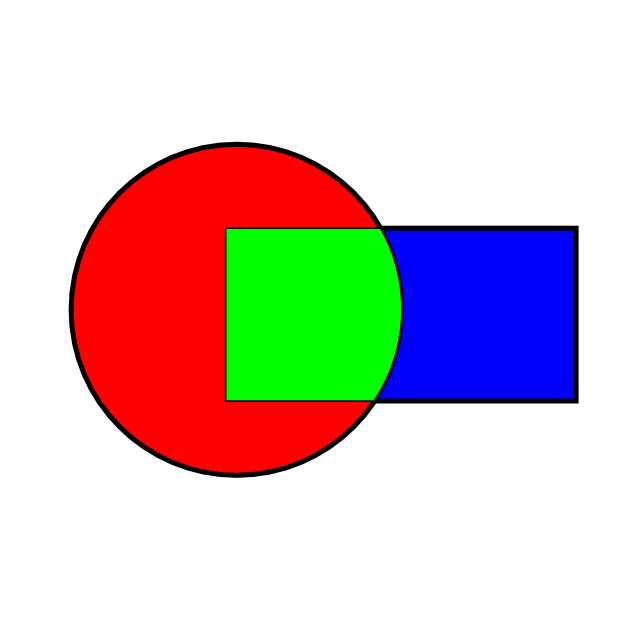
- The method of parallel computing used by OpenFOAM, and CFD in general, is known as domain decomposition.
- Domain Decomposition Methods (DDM) are a specialized field of mathematics and computational science, http://www.ddm.org
-
In DDM, geometry and associated fields are broken into pieces and allocated to separate processors for solution.
Parallel Utilities
To support DDM in OpenFOAM, there are 4 parallel processing utilities:
[03:03:53][egp@egpMBP:parallelProcessing]542$ pwd
/Users/egp/OpenFOAM/OpenFOAM-2.2.x/applications/utilities/parallelProcessing
[03:04:09][egp@egpMBP:parallelProcessing]543$ ls -l
total 0
drwxr-xr-x  3 egp  staff  918 May 17 09:51 decomposePar
drwxr-xr-x  3 egp  staff  204 May 17 09:51 reconstructPar
drwxr-xr-x  3 egp  staff  170 May 17 09:52 reconstructParMesh
drwxr-xr-x  3 egp  staff  272 May 17 09:52 redistributePar
Process
- Case preparation
- Parallel executation
- Data analysis and visualization
- Reconstruction, only for special cases
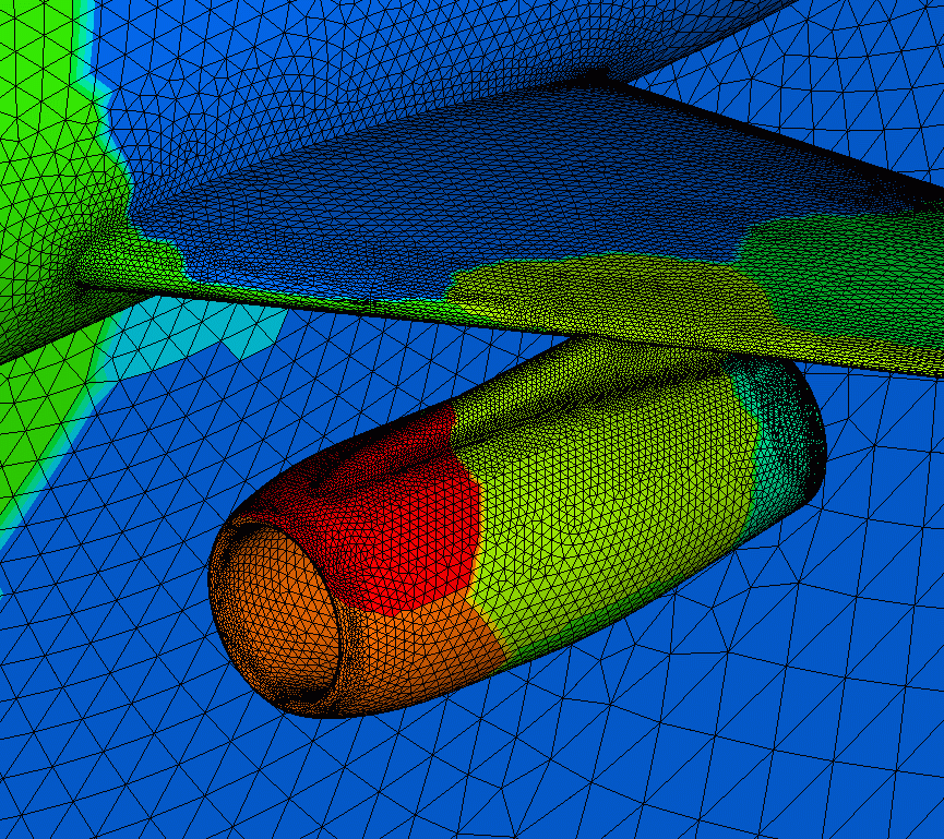
Case Preparation
- Typically, the case will be prepared in one piece: serial mesh generation
- decomposePar: parallel decomposition tool, controlled by the dictionary decomposeParDict
- Options in the dictionary allow choice of decomposition and auxiliary data
- Upon decomposition, processorNN directories are created with decomposed mesh and fields; solution controls, model choice and discretization parameters are shared. Each CPU may use local disk space, however, on BlueRidge, disk space is shared across all compute nodes
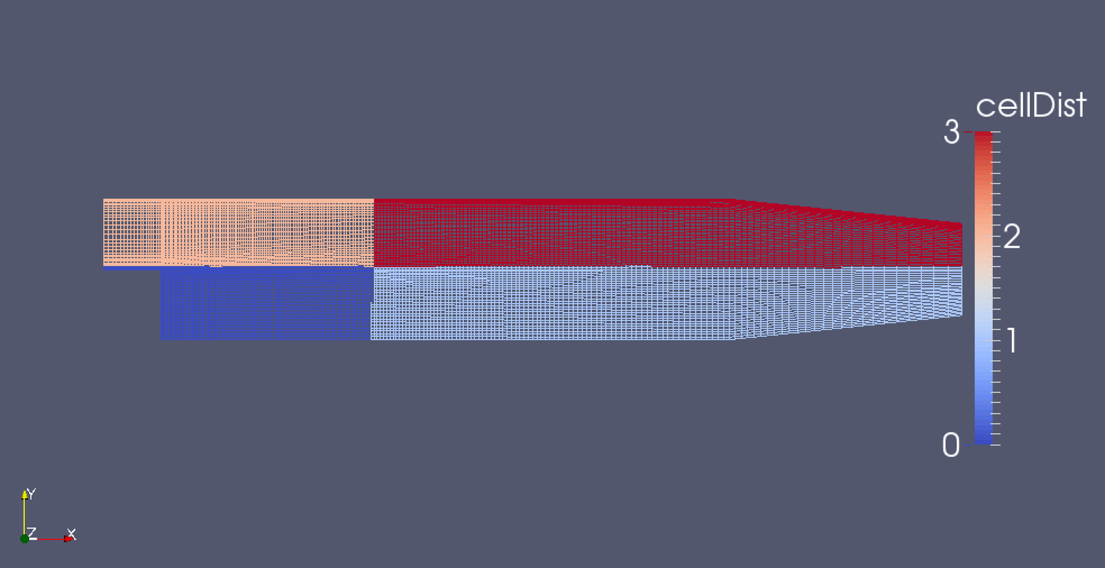
- decomposePar -cellDist writes cell-to-processor decomposition for visualization
decomposePar
- The goal of decomposition is to break up the domain with minimal effort but in such a way to guarantee a fairly economic solution (i.e., load balanced).
- The geometry and fields are decomposed according to a set of parameters specified in a dictionary named decomposeParDict that must be located in the system directory.
- In the decomposeParDict file the user must set the number of domains which the case should be decomposed into: usually it corresponds to the number of cores available for the calculation.
- For example, on BlueRidge, where we have 16-cores/node, a 4-node simulation would result in 64-processors and Subdomains
-
numberOfSubdomains 64;
decomposePar
- The user has a choice of seven methods of decomposition, specified by the method keyword.
- For each method there are a set of coefficients specified in a sub-dictionary of decompositionDict, named
<method>Coeffs, used to instruct the decomposition process: - simple: simple geometric decomposition in which the domain is split into pieces by direction, e.g. 2 pieces in the x direction, 1 in y etc.
- hierarchical: Hierarchical geometric decomposition which is the same as simple except the user specifies the order in which the directional split is done, e.g. first in the y-direction, then the x-direction etc.
decomposePar
- metis: METIS decomposition which requires no geometric input from the user and attempts to minimize the number of processor boundaries. The user can specify a weighting for the decomposition between processors which can be useful on machines with differing performance between processors.
- scotch: similar technology as metis, and with a more flexible open-source license, http://www.labri.fr/perso/pelegrin/scotch/
- manual: Manual decomposition, where the user directly specifies the allocation of each cell to a particular processor.
- multilevel: similar to hierarchical, but all methods can be used in a nested form
- structured: special case.
pitzDailyParallel
-
copy pitzDaily tutorial and use as example
- copy boilerplate decomposeDict from $FOAM_UTILITIES
[03:41:22][egp@brlogin1:simpleFoam]13058$ cp -rf pitzDaily pitzDailyParallel[03:42:42][egp@brlogin1:pitzDailyParallel]13066$ cp $FOAM_UTILITIES/parallelProcessing/decomposePar/decomposeParDict system/.
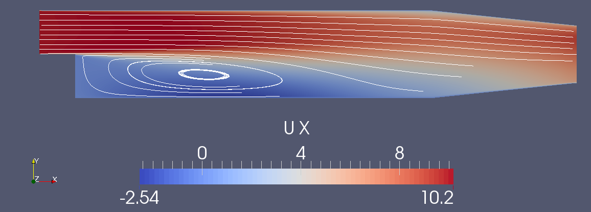
pitzDaily Backward Facing Step tutorial
pitzDailyParallel
output from decomposePar
code text box below is scrollable. hover mouse, and scroll
[05:12:36][egp@brlogin1:pitzDailyParallel]13097$ decomposePar -cellDist
/*---------------------------------------------------------------------------*\
| =========                 |                                                 |
| \\      /  F ield         | OpenFOAM: The Open Source CFD Toolbox           |
|  \\    /   O peration     | Version:  2.2.0                                 |
|   \\  /    A nd           | Web:      www.OpenFOAM.org                      |
|    \\/     M anipulation  |                                                 |
\*---------------------------------------------------------------------------*/
Build  : 2.2.0
Exec   : decomposePar -cellDist
Date   : Nov 14 2013
Time   : 05:12:46
Host   : "brlogin1"
PID    : 61396
Case   : /home/egp/OpenFOAM/egp-2.2.0/run/tutorials/incompressible/simpleFoam/pitzDailyParallel
nProcs : 1
sigFpe : Floating point exception trapping - not supported on this platform
fileModificationChecking : Monitoring run-time modified files using timeStampMaster
allowSystemOperations : Disallowing user-supplied system call operations

// * * * * * * * * * * * * * * * * * * * * * * * * * * * * * * * * * * * * * //
Create time


Decomposing mesh region0

Removing 4 existing processor directories
Create mesh

Calculating distribution of cells
Selecting decompositionMethod scotch

Finished decomposition in 0.07 s

Calculating original mesh data

Distributing cells to processors

Distributing faces to processors

Distributing points to processors

Constructing processor meshes

Processor 0
    Number of cells = 3056
    Number of faces shared with processor 1 = 86
    Number of faces shared with processor 2 = 60
    Number of processor patches = 2
    Number of processor faces = 146
    Number of boundary faces = 6222

Processor 1
    Number of cells = 3056
    Number of faces shared with processor 0 = 86
    Number of processor patches = 1
    Number of processor faces = 86
    Number of boundary faces = 6274

Processor 2
    Number of cells = 3065
    Number of faces shared with processor 0 = 60
    Number of faces shared with processor 3 = 57
    Number of processor patches = 2
    Number of processor faces = 117
    Number of boundary faces = 6237

Processor 3
    Number of cells = 3048
    Number of faces shared with processor 2 = 57
    Number of processor patches = 1
    Number of processor faces = 57
    Number of boundary faces = 6277

Number of processor faces = 203
Max number of cells = 3065 (0.286299% above average 3056.25)
Max number of processor patches = 2 (33.3333% above average 1.5)
Max number of faces between processors = 146 (43.8424% above average 101.5)


Wrote decomposition to "/home/egp/OpenFOAM/egp-2.2.0/run/tutorials/incompressible/simpleFoam/pitzDailyParallel/constant/cellDecomposition" for use in manual decomposition.

Wrote decomposition as volScalarField to cellDist for use in postprocessing.
Time = 0

Processor 0: field transfer
Processor 1: field transfer
Processor 2: field transfer
Processor 3: field transfer

End.
Scotch Decomposition
method          scotch;scotchCoeffs
{
} 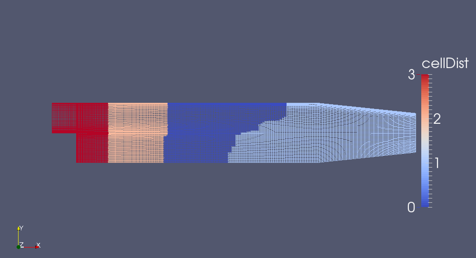
simple Decomposition
method          simple;simpleCoeffs
{
 (2 2 1);
    delta         n
   0.001;
}
Parallel Execution
- Top-level code does not change between serial and parallel execution: operations related to parallel support are embedded in the library
- Launch executable using mpirun with -parallel option
- Data in time directories is created on a per-processor basis
mpirun -np $PBS_NP simpleFoam -parallel 2>&1 | tee log.simpleFoam
- $PBS_NP is an environment variable that holds the number of requested cores
- mpirun is an application that launches the parallel job and farms out the tasks to the cores listed in $PBS_NODEFILE
Parallel Performance
-
In Homework #2, you will need to perform a parallel performance study.
- To increase the size of your mesh, edit the constant/polyMesh/blockMeshDict and increase the number in each direction. BE CAREFUL! This is fragile!
blocks
(
    hex (0 6 7 1 22 28 29 23) (18 7 1) simpleGrading (0.5 1.8 1)
    hex (1 7 8 2 23 29 30 24) (18 10 1) simpleGrading (0.5 4 1)
    hex (2 8 9 3 24 30 31 25) (18 13 1) simpleGrading (0.5 0.25 1)
    hex (4 10 11 5 26 32 33 27) (180 18 1) simpleGrading (4 1 1)
    hex (5 11 12 6 27 33 34 28) (180 9 1) edgeGrading (4 4 4 4 0.5 1 1 0.5 1 1 1 1)
    hex (6 12 13 7 28 34 35 29) (180 7 1) edgeGrading (4 4 4 4 1.8 1 1 1.8 1 1 1 1)
    hex (7 13 14 8 29 35 36 30) (180 10 1) edgeGrading (4 4 4 4 4 1 1 4 1 1 1 1)
    hex (8 14 15 9 30 36 37 31) (180 13 1) simpleGrading (4 0.25 1)
    hex (10 16 17 11 32 38 39 33) (25 18 1) simpleGrading (2.5 1 1)
    hex (11 17 18 12 33 39 40 34) (25 9 1) simpleGrading (2.5 1 1)
    hex (12 18 19 13 34 40 41 35) (25 7 1) simpleGrading (2.5 1 1)
    hex (13 19 20 14 35 41 42 36) (25 10 1) simpleGrading (2.5 1 1)
    hex (14 20 21 15 36 42 43 37) (25 13 1) simpleGrading (2.5 0.25 1)
);
blockMesh set-up
-
blockMesh is a simple algebraic mesh generator in OpenFOAM
- It requires that you have a map of the point and blocks
- This is important when adjusting mesh size for parallel performance studies
- To generate a new mesh, run blockMesh

Data Analysis
- Post-processing utilities, including sampling tools, will execute correctly in parallel, e.g.,
- mpirun -np $PBS_NP vorticity -parallel
- mpirun -np $PBS_NP Q -parallel
- mpirun -np $PBS_NP sample -parallel
- etc.
- This is VERY IMPORTANT for large simulations. You want to avoid reconstruction, because:
- It is time consuming
- It duplicates large datasets and uses a lot of disk space
sample utility for PitzDaily
- sample utility can do many things
- set sampling along lines and clouds
- surface sampling on planes, patches, isoSurfaces, and specified triangulated surfaces
- Allows you to focus on light-weight data vs. entire dataset!!
- To start, copy the boilerplate sampleDict from $FOAM_UTILITIES
- As an example, let's sample pitzDaily along the centerline and a vertical profile, and surface which is a uniform distance from the wall. Next slides describe the modifications.
-
Then run sample in parallel
cp $FOAM_UTILITIES/postProcessing/sampling/sample/sampleDict system/.
mpirun -np 4 sample -latestTime -parallel
sampleDict
sample velocity, pressure, and turbulence variables
fields
(
    p
    U
    nut
    k
    epsilon
);
surfaces
(
nearWalls_interpolated
{
// Sample cell values off patch. Does not need to be the near-wall
// cell, can be arbitrarily far away.
type patchInternalField;
patches ( ".*Wall.*" );
interpolate true;
offsetMode normal;
distance 0.0001;
}
); sampleDict, cont.
sets
(
    centerline
    {
        type        midPointAndFace;
        axis        x;
        start       (0.0 0.0 0.0);
        end         (0.3 0.0 0.0);
    }
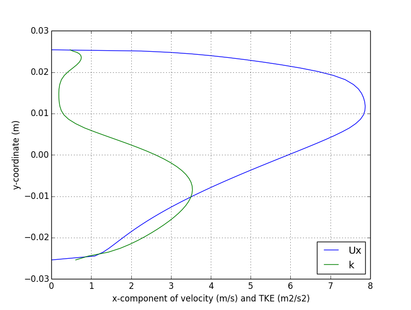
    verticalProfile
    {
        type        midPointAndFace;
        axis        y;
        start       (0.206 -0.03 0.0);
        end         (0.206  0.03 0.0);
    }
);
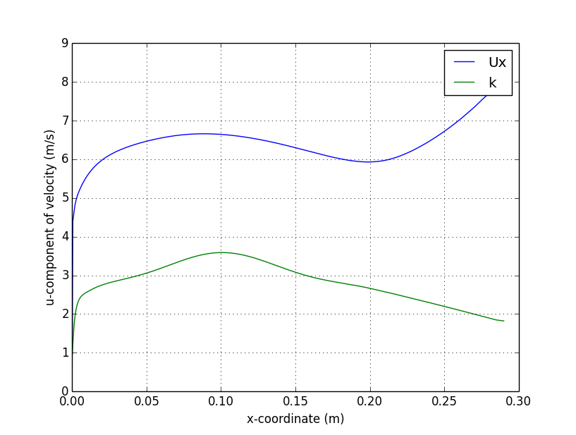
Centerline plot
Vertical Profile plot
Near-wall surfaces
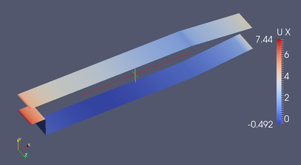
Axial velocity
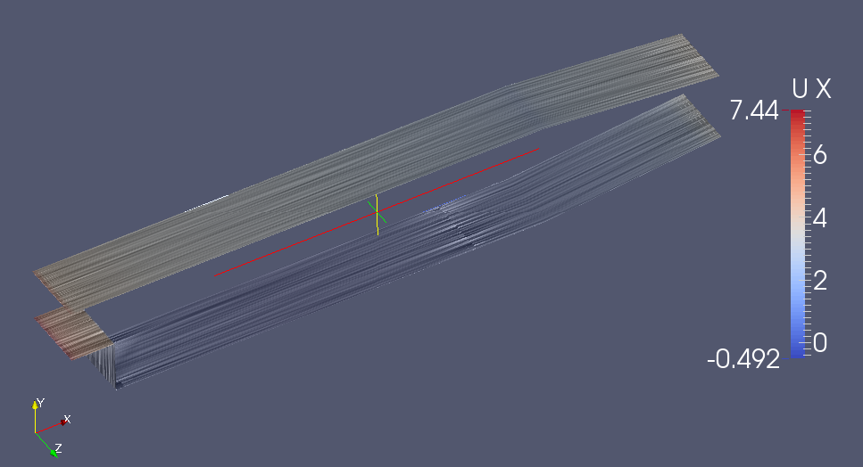
Surface oil streamlines using line-integral convolution (LIC)
Visualization
- Most common visualization tools read parallel OpenFOAM data: Paraview, Tecplot, Ensight, Fieldview. Again, avoid the use of reconstructPar
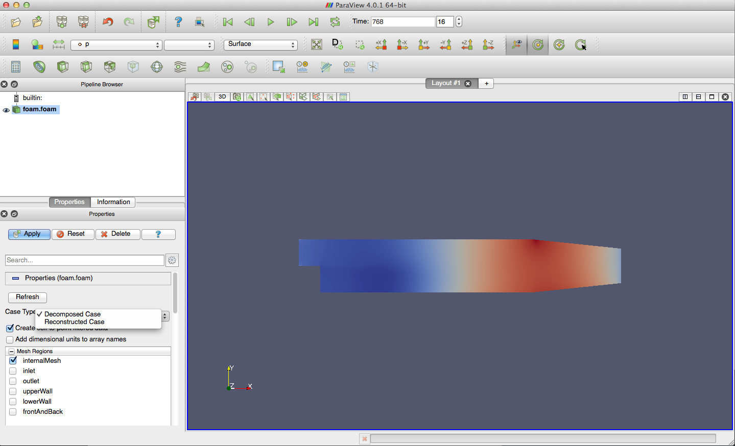
next lecture: more Data Analysis and Visualization
