Inferential

Statistics

What is the amount of time spend by our customers on the web ?

Who will win the next election ?

Do we need to change the process mechanism or we are doing thing efficiently ?

What are our order lead times post recent vendor engagement for supplies ?

What is the air quality level today ?

Is the new drug proving effective ?

Population

Total collection of objects or people to be studied (or set of all information of interest to the decision maker)

Sample

Statistical Inference

Making statements about a population parameter on the basis of a sample statistic

Subset of Population

What is sampling?
Using subsets of a target population to assess population characteristics of interest.
 

Key principle underlying sampling?
A suitable subset of a target population can adequately describe
population characteristics.
 

Why care about sampling?
– Because the alternatives are worse.
– Census taking may be prohibitively expensive, or, even impossible.
– That leaves making judgment calls without a solid basis in data.
 

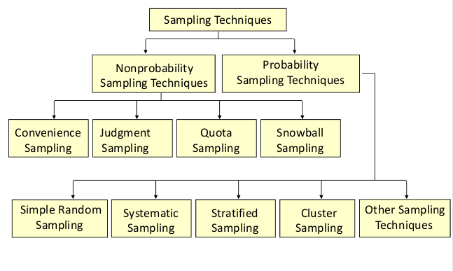
Sampling : Two Principal Approaches

Probability Sampling

Non-Probability Sampling

In Probability Sampling, every member of the population has a known or calculable
probability of being included in the sample.

The main advantage is that

(i) Error margins on sample statistic are computable for a given sample size

(ii) Generalization of statistical analysis to the population feasible.

Non-Probability Sampling is everything that is not Probability sampling. None of
the advantages pertain, either.

However, it is done because either

(i) Probability samples are infeasible in a particular case, or

(ii) qualitative research is being done; this does not need Probability samples, Or

(iii) the target population is relatively small (e.g. some B2B contexts).

Probability sampling is a sampling technique wherein the samples are gathered in a process that gives all the individuals in the population equal chances of being selected.

A researcher must identify specific sampling elements (e.g. persons) to include in the sample.

For example, if conducting a telephone survey, the researcher needs to try to reach the specific sampled person, by calling back several times, to get an accurate sample

Probability Sampling Methods

Random Sample : The term random has a very precise meaning. Each individual in the population of interest has an equal likelihood of selection. This is a very strict meaning -- you can't just collect responses on the street and have a random sample.

The assumption of an equal chance of selection means that sources
such as a telephone book or voter registration lists are not adequate for providing a random sample of a community. In both these cases there will be a number of residents whose names are not listed.

Telephone surveys get around this problem by random-digit dialing -- but that assumes that everyone in the population has a telephone.

The key to random selection is that there is no bias involved in the selection of the sample. Any variation between the sample characteristics and the population characteristics is only a matter of chance.

A stratified sample is a mini-reproduction of the population.

• If the population is not homogeneous, SRS is not very effective.
• Therefore, the entire population is divided into several homogeneous groups (strata) according to the characteristics of importance for the research (e.g. by gender, social class, blood group, education level, etc)
• Then the population is randomly sampled within each category or
stratum. If 38% of the population is college-educated, then 38% of the sample is randomly selected from the college-educated population.
• Stratified samples are as good as or better than random samples, but they require a fairly detailed advance knowledge of the population characteristics, and therefore are more difficult to construct.

Cluster sampling is a sampling technique used when "natural" but
relatively homogeneous groupings are evident in a statistical population.

It is often used in marketing research.

In this technique, the total population is divided into these groups (or clusters) and a simple random sample of the groups is selected.

Non Probability Sampling Methods

• As they are not truly representative, non-probability samples are less desirable than probability samples. However, a researcher may not be able to obtain a random or stratified sample, or it may be too expensive.

• A researcher may not care about generalizing to a larger population.

• The validity of non-probability samples can be increased by trying to approximate random selection, and by eliminating as many sources of bias as possible.

Non Probability Sampling

• The defining characteristic of a quota sample is that the researcher
deliberately sets the proportions of levels or strata within the sample. This is generally done to insure the inclusion of a particular segment of the population.

• The proportions may or may not differ dramatically from the actual
proportion in the population. The researcher sets a quota, independent of population characteristics.

Quota Sampling

Convenience sampling is a sample taken from a group you have easy access to. The idea is that anything learned from this study will be applicable to the larger population.

• By using a large, convenient size, you are able to more confidently say the sample represents the population.

• Furthermore, the convenient group you are testing should not be
fundamentally different than if you had taken a sample from another
area. If you are trying to say something about women, for example,
then your convenient sample cannot be men.

Judgment sample is a type of nonrandom sample that is selected
based on the opinion of an expert.

• Results obtained from a judgment sample are subject to some degree of bias, due to the frame and population not being identical.

• The frame is a list of all the units, items, people, etc., that define the population to be studied.

•Example: A TV researcher wants a quick sample of opinions about a political announcement. Taking views of people in the street.

3 Main Sampling Techniques

• Simple Random Sample
• Systematic
• Stratified

Simple Random Sample

• Unbiased: Each unit has equal chance of being chosen in the sample
• Independent: Selection of one unit has no influence on selection of other units
• SRS is a gold standard against which all other samples are measured

Simple Random Sample

• Advantages:
  • Can be used with large sample populations
  • Avoids bias
• Disadvantages:
  • Can lead to poor representation of the overall parent population or area if large areas are not hit by the random numbers generated. This is made worse if the study area is very large
  • There may be practical constraints in terms of time available and access to certain parts of the study area

• Samples are chosen in a systematic, or regular way.

• They are evenly/regularly distributed in a spatial context, for example every two meters along a transect line.

• They can be at equal/regular intervals in a temporal context, for example every half hour or at set times of the day.

• They can be regularly numbered, for example every 10th house or
person

Systematic Sampling

Advantages:
• It is more straight-forward than random sampling
• A grid doesn't necessarily have to be used, sampling just has to be at uniform intervals
• A good coverage of the study area can be more easily achieved than using random sampling

Disadvantages:
• It is more biased, as not all members or points have an equal chance of being selected
• It may therefore lead to over or under representation of a particular pattern

Systematic Sampling

Stratified Sampling

This method is used when the parent population or sampling frame
is made up of sub-sets of known size.

These sub-sets make up different proportions of the total, and therefore sampling should be stratified to ensure that results are proportional and representative of the whole.

Stratified Sampling

Advantages:
• It can be used with random or systematic sampling, and with point,
line or area techniques
• If the proportions of the sub-sets are known, it can generate results which are more representative of the whole population
• It is very flexible and applicable to many geographical enquiries
• Correlations and comparisons can be made between sub-sets

Disadvantages:
• The proportions of the sub-sets must be known and accurate if it is to work properly
• It can be hard to stratify questionnaire data collection, accurate up to date population data may not be available and it may be hard to identify people's age or social background effectively

Selecting the Sampling Frame

Sampling frame is simply a list of items from which to draw a sample

Does the sampling frame represent the population?
– e.g. Literary Digest vs. George Gallup polls

 

Roosevelt’s ultimate victory “led to the death of the Literary Digest“ and helped make Gallup “a household name.”

CASE 1

CASE 2

During World War II, Wald was a member of the Statistical Research Group (SRG) where he applied his statistical skills to various wartime problems. These included methods of sequential analysis and sampling inspection.

One of the problems that the SRG worked on was to examine :

the distribution of damage to aircraft to provide advise on how to minimize bomber losses to enemy fire.

There was a inclination within the military to consider providing greater protection to parts that received more damage but.....

CASE 2

Wald made the assumption that damage must be more uniformly distributed and that the aircraft that did return or show up in the samples were hit in the less vulnerable parts.

Wald noted that

- the study only considered the aircraft that had survived their missions

- the bombers that had been shot down were not present for the damage assessment.

The holes in the returning aircraft, then, represented areas where a bomber could take damage and still return home safely.

Wald proposed that the Navy instead reinforce the areas where the returning aircraft were unscathed, since those were the areas that, if hit, would cause the plane to be lost. 

His work is considered seminal in the then-fledgling discipline of operational research.

Sometimes, no comprehensive sampling frame exists

– e.g. when forecasting for the future. Thus a comprehensive list of acceptances of credit card offers does not exist yet

Typical Pitfalls in Sampling

Collecting data only from volunteers (voluntary response sample)

– e.g. online reviews (yelp.com, maps.google.com, tripadvisor.com)

Picking easily available respondents (convenience sample)

– e.g. choosing to survey in Ambience mall

A high rate of non‐response (more than 70%)

– e.g. CEO / CIO surveys on some industry trends

Sampling Variance

Sample mean varies from one sample to another

• Sample mean can be (and most likely is) different from the population mean

• Sample mean is a random variable

Sample statistics and Population parameters

Central Limit Theorem (CLT)

&

The distribution of the sample mean

The central limit theorem (CLT) is a statistical theory that states that given a sufficiently large sample size from a population with a finite level of variance,

- Sampling distribution of the sampling means approaches a normal distribution as the sample size gets larger - no matter what the shape of the population distribution. This fact holds especially true for sample sizes over 30.

- the mean of all samples from the same population will be approximately equal to the mean of the population.

Mean (    ) = μ (the same as the population mean of the raw data)

Standard deviation (    )  =          , where σ is the population standard deviation and n is the
sample size
– This is referred to as Standard Error of the Mean

CLT is valid when ...

• Each data point in the sample is independent of the other
• The sample size is large enough

How Large is Large Enough?

Depends on distribution of data – primarily its symmetry and presence of outliers
• If data is quite symmetric and has few outliers, even smaller samples are fine. Otherwise, we need larger samples
• A sample size of 30 is considered large enough, but that may/ may not be adequate
• More precise conditions
– n > 10 (K 3 ) 2 , where K 3  is sample skewness, and
– n > 10 |K 4 |, where K 4  is sample kurtosis

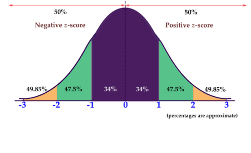
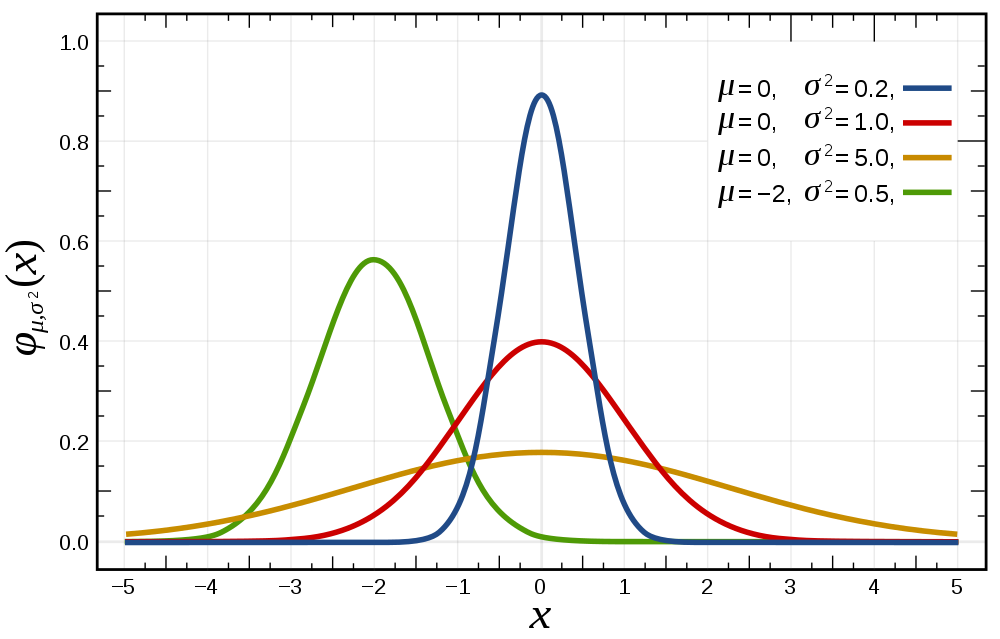
Normal Distribution

• The graph of the pdf (probability density function) is a bell shaped curve.
• The normal random variable takes values from ‐ ∞ to +∞
• It is symmetric and centered around the mean (which is also the median and mode)
• Any normal distribution can be specified with just two parameters – the mean (μ) and the standard deviation (σ)

We write this as X~N(μ,σ 2 )

Many things closely follow a Normal Distribution:

• Heights of people
• Size of things produced by machines
• Errors in measurements
• Blood pressure
• Marks on a test

Probability Calculation for Continuous Distributions

The probability associated with any single value of the random variable is always ______

Probability Calculation for Continuous Distributions

The probability associated with any single value of the random variable is always zero

Probability of values being in a range = ____ under the pdf curve in that range

Probability Calculation for Continuous Distributions

The probability associated with any single value of the random variable is always zero

Probability of values being in a range = Area under the pdf curve in that range

Area under the entire curve always equals ___

Probability Calculation for Continuous Distributions

The probability associated with any single value of the random variable is always zero

Probability of values being in a range = Area under the pdf curve in that range

Area under the entire curve always equals 1

Z Score

or

Standard Score

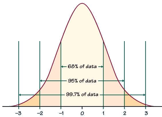
The Standard Deviation is a measure of how spread out numbers are.

When we calculate the standard deviation we find that (generally):

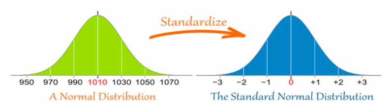
Standard Scores

The number of standard deviations from the mean is also called the "Standard Score", "sigma" or "z-score". Get used to those words!

So to convert a value to a Standard Score ("z-score"):
• first subtract the mean,
• then divide by the Standard Deviation
• And doing that is called "Standardizing"
• We can take any Normal Distribution and convert it to The
Standard Normal Distribution.

Travel Time

A survey of daily travel time had these results (in minutes):
26, 33, 65, 28, 34, 55, 25, 44, 50, 36, 26, 37, 43, 62, 35, 38, 45, 32,
28, 34

Mean ?

Standard Deviation ?

Z scores ?

Estimation

• In statistics, estimation refers to the process by which one makes
inferences about a population, based on information obtained from a sample.

• An estimator attempts to approximate the unknown parameters using the measurements.

• For example, it is desired to estimate the proportion of a population of voters who will vote for a particular candidate.

•That proportion is the parameter sought; the estimate is based on
a small random sample of voters.

• Estimation is the process of determining a likely value for a population parameter (e.g. the true population mean or proportion) based on a random sample.

• In practice, a sample is drawn from the target population, and
sample statistics (e.g. the sample mean or sample proportion) are
used to generate estimates of the unknown parameter.

• The sample should be representative of the population, ideally
with participants selected at random from the population.

• Because different samples can produce different results, it is
necessary to quantify the sampling error or variation that exists
among estimates from different samples.

You are a middle school principal and your 100 eighth-graders are
about to take a national standardized test. The test is designed so
that the mean score is μ = 400 with a standard deviation of σ = 70.
Assume the scores are normally distributed.

What is the likelihood that one of your eighth-graders, selected at
random, will score below 375 on the exam?

Predicting Test Scores : Problem 1

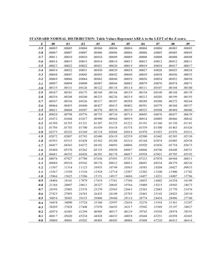
Since the distribution is normal, we can just use z-scores to
determine the percentage for one student

z =  (375 - 400)/70 = - 0.36
 

According to the standard normal distribution table, a z-score of -0.36 corresponds to about 36%

Which means that about 36% of all students can be expected to score below 375, thus there is a 36% chance that a randomly selected student will score below 375

Predicting Test Scores : Problem 1

Predicting Test Scores : Problem 1+

Your performance as a principal depends on how well your entire
group of eighth-graders scores on the exam. What is the likelihood
that your group of 100 eighth-graders will have Mean score below
375?

According to the C.L.T. if we take random groups of say 100 students
and study their means, then the means distribution will approach
normal.

Hence, the μ = 400 and its standard deviation is

σ/√n = 70/√100 = 70/10 = 7

according to the C.L.T . Therefore, the z-score for a mean of 375 with a standard deviation of 7 is:

z = (375 - 400)/7 = 3.57

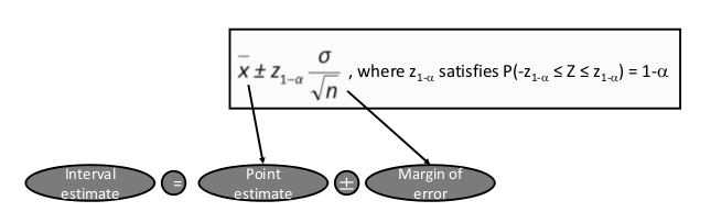
Point & Interval Estimates

• The point estimate is our best guess of the true value of the parameter, while the interval estimate gives a measure of accuracy of that point estimate by providing an interval that contains plausible values.

• Point estimate: A point estimate of a population parameter is a single value of a statistic.

• For example, the sample mean x is a point estimate of the
population mean Similarly , the sample proportion p is a point
estimate of the population proportion P.

Interval estimate:

An interval estimate is defined by two numbers, between which a
population parameter is said to lie.

• For example, a < x < b is an interval estimate of the population
mean μ.

It indicates that the population mean μ is greater than "a" but less than "b".

Problem
Find a point estimate of mean university student height with the
sample data from survey.
 

Solution
For convenience, we begin with storing the survey data of student
heights in the variable height. Survey.

It turns out not all students have answered the question, and we
must filter out the missing values.

library(MASS)
MH <- mean(survey$Height)
MH

Hence we apply the mean function with the "na.rm" argument
as TRUE for skipping the missing values.

A point estimate of the mean student height is 172.38 centimeters.

library(MASS)
MH <- mean(survey$Height, na.rm = TRUE)
MH

Interval Estimates

A university with 100,000 alumni is thinking of offering a new affinity credit card to its alumni.

• Profitability of the card depends on the average balance maintained by the cardholders.

• A market research campaign is launched, in which about 140 alumni accept the card in a pilot launch.

• Average balance maintained by these is $1990 and the standard deviation is $2833. Assume that the population standard deviation is $2500 from previous launches.

• What can we say about the average balance that will be held after a full‐fledged market launch?

Based on the sample data:

– The point estimate for mean balance = $1990
– Can we trust this estimate?
 

Based on the sample data:

– The point estimate for mean balance = $1990
– Can we trust this estimate?
 

What do you think will happen if we took another random sample of 140 alumni?

Because of this uncertainty, we prefer to provide the estimate as an interval (range) and associate a level of confidence with it

Interval Estimate  :  Point Estimate  ±  Margin of Error

How big should be the Margin Of Error ?

Trade‐off between level of confidence and accuracy

Sample Mean ~ Population Mean

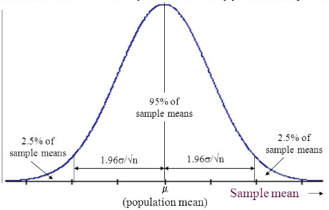
Assume that sample size is large enough so that CLT can be applied.

The distribution of the sample means is
 

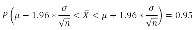
From normal distribution calculations, 95% of all possible sample means will lie within 1.96 SE of the population mean

 ~ N( μ ,              )

If we have to make a statement about an
unknown but constant μ based on the
mean  X bar of a random sample

Interpretation 1: Mean of the population
has a 95% chance of being in this range
for a random sample

Interpretation 2: Mean of the population
will be in this range for 95% of random
samples

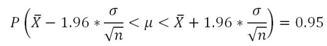
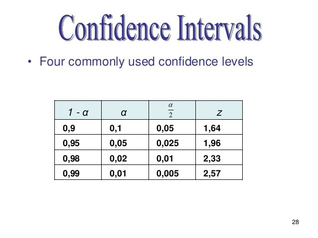
Start by choosing a confidence level (1‐α)% (e.g. 95%, 99%, 90%)

Then, the population mean will be within

Margin of error depends on the underlying uncertainty, confidence level and the sample size

Interval Estimate of Population Mean-Known Variance

Based on the survey and past data
n = 140; σ = $ 2500;     Xbar = $ 1,990

Margin Of Error = 2500/sqrt(140) = 211.29

• Construct a 95% confidence interval for the mean card balance and interpret it

• Construct a 90% confidence interval for the mean card balance and interpret it

Credit Card : Mean Balance

Problem
Assume the population standard deviation σ of the student height
in survey is 9.48. Find the margin of error and interval estimate at
95% confidence level.

Solution
We first filter out missing values in survey$Height with the na.omit function, and save it in height.response.

Then we compute the standard error of the mean.

n = dim(survey)[1] - sum(is.na(survey$Height))
sigma = 9.48
SEMean = sigma/sqrt(n)
SEMean

Since there are two tails of the normal distribution, the 95%
confidence level would imply the 97.5th percentile of the normal
distribution at the upper tail. Therefore, in R, zα∕ is given by
qnorm(.975).

We multiply it with the standard error of the mean and get the
margin of error.

# Marging of Error
ME = qnorm(0.975)*SEMean
ME

We then add it up with the sample mean, and find the confidence
interval as told.

MH+c(ME,-ME) 

Assuming the population standard deviation σ being 9.48, the margin of error for the student height survey at 95% confidence level is 1.2852 centimeters. The confidence interval is between 171.10 and 173.67 centimeters.

(Mis)Interpreting the Confidence Interval
 

Consider the 95% Confidence Interval for the mean height : [171.10, 173.67]

Does this mean that :

A The mean height of the population lies in this range?

B The mean height is in this range 95% of the time?

C 95% of the population have height in this range?

Data Visualisation

(Appetizer) >>

Thank You