Modeling Topological Polymers

Collaborators


Jason Cantarella
U. of Georgia
Tetsuo Deguchi
Ochanomizu U.
Erica Uehara
Ochanomizu U.
Funding: Simons Foundation
Linear polymers
A linear polymer is a chain of molecular units with free ends.
Polyethylene


Nicole Gordine [CC BY 3.0] from Wikimedia Commons
Shape of linear polymers
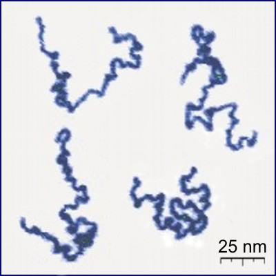
In solution, linear polymers become crumpled:
Protonated P2VP
Roiter–Minko, J. Am. Chem. Soc. 127 (2005), 15688-15689
[CC BY-SA 3.0], from Wikimedia Commons
Ring polymers
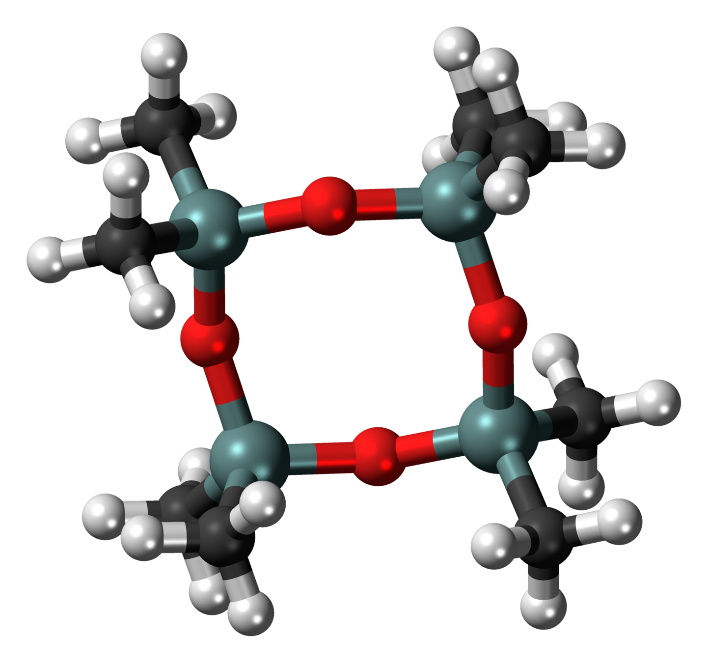
Octamethylcyclotetrasiloxane
(Common in cosmetics, bad for fish)
Ring biopolymers
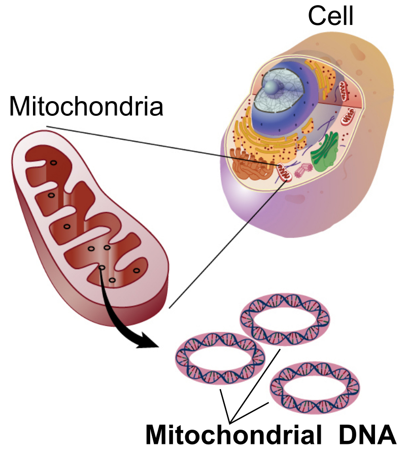
Most known cyclic polymers are biological
Material properties
Ring polymers have weird properties; e.g.,
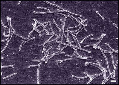
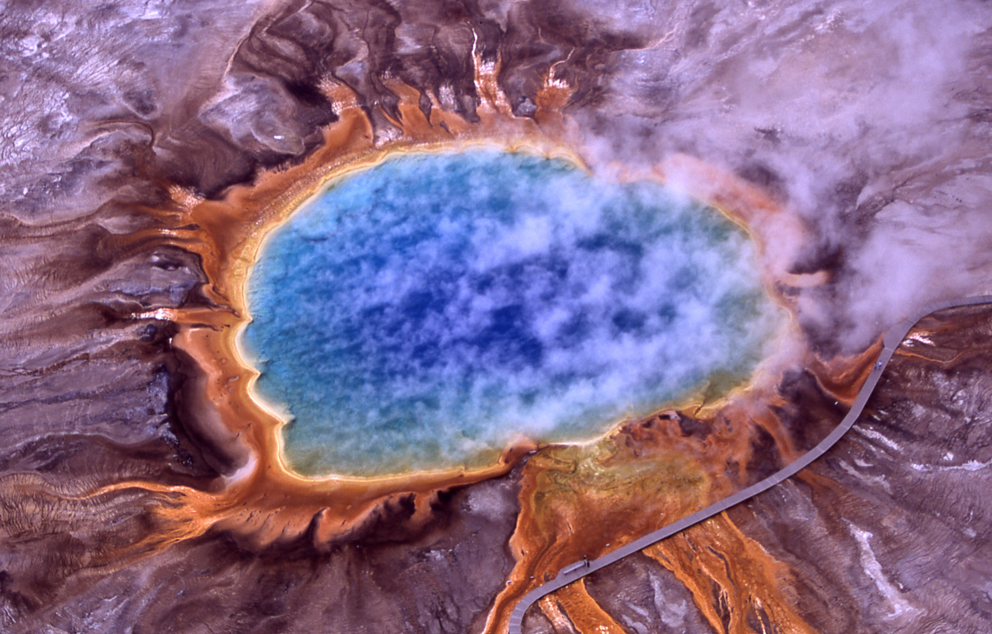
Thermus aquaticus
Uses cyclic archaeol, a heat-resistant lipid
Grand Prismatic Spring
Home of t. aquaticus; 170ºF
Topological polymers
A topological polymer joins monomers in some graph type:
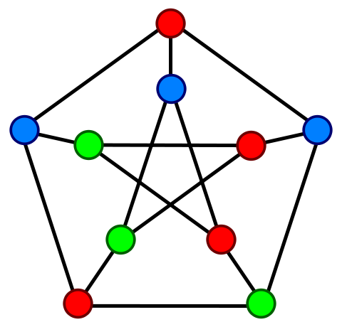
Petersen graph
In biology
Topological biopolymers have graph types that are extremely complicated (and thought to be random):
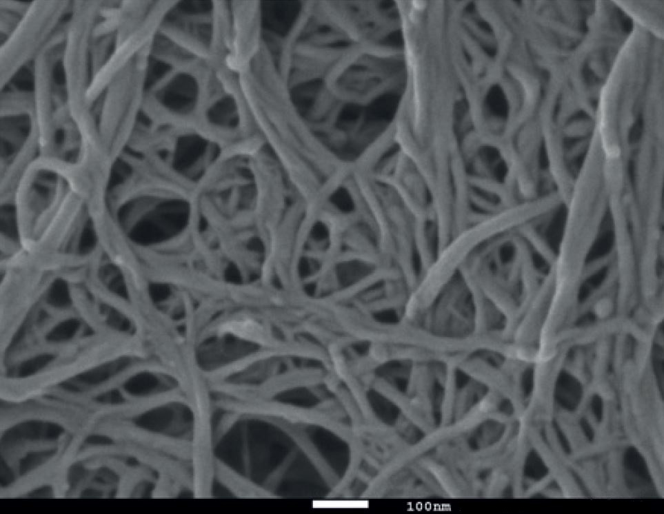
Wood-based nanofibrillated cellulose
Qspheroid4 [CC BY-SA 4.0], from Wikimedia Commons
Synthetic topological polymers
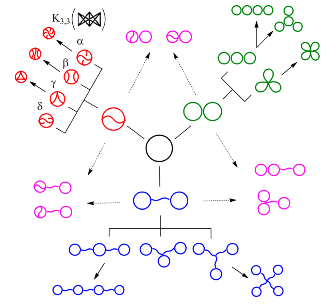
The Tezuka lab in Tokyo can now synthesize many topological polymers in usable quantities
Y. Tezuka, Acc. Chem. Res. 50 (2017), 2661–2672
Main Question
What is the probability distribution on the shapes of topological polymers in solution?
Ansatz
Linear polymers
Ring polymers
Topological polymers
Random walks with independent steps
Random walks with steps conditioned on closure
Random walks with steps conditioned on ???
Functions and vector fields
Suppose \(\mathfrak{G}\) is a directed graph with \(\mathfrak{V}\) vertices and \(\mathfrak{E}\) edges.
Definition. A function on \(\mathfrak{G}\) is a map \(f:\{v_1,\dots , v_\mathfrak{V}\} \to \mathbb{R}\). Functions are vectors in \(\mathbb{R}^\mathfrak{V}\).
Definition. A vector field on \(\mathfrak{G}\) is a map \(w:\{e_1,\dots , e_\mathfrak{E}\} \to \mathbb{R}\). Vector fields are vectors in \(\mathbb{R}^\mathfrak{E}\).
Gradient and divergence
By analogy with vector calculus:
Definition. The gradient of a function \(f\) is the vector field
Definition. The divergence of a vector field \(w\) is the function
Gradient and divergence as matrices
So if \(B = \operatorname{div}\), which is \(\mathfrak{V} \times \mathfrak{E}\), then \(\operatorname{grad} = B^T\).
Helmholtz’s Theorem
Fact.
The space \(\mathbb{R}^\mathfrak{E}\) of vector fields on \(\mathfrak{G}\) has an orthogonal decomposition
Corollary.
A vector field \(w\) is a gradient (conservative field) if and only if the (signed) sum of \(w\) around every loop in \(\mathfrak{G}\) vanishes.
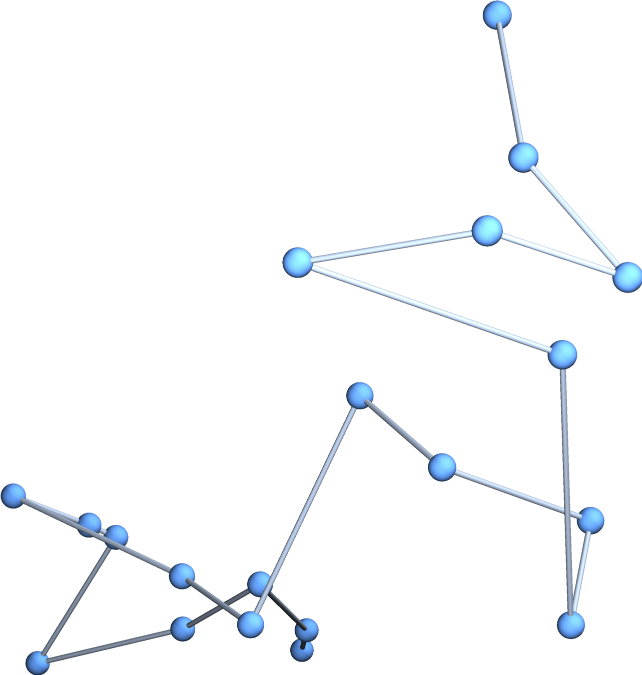
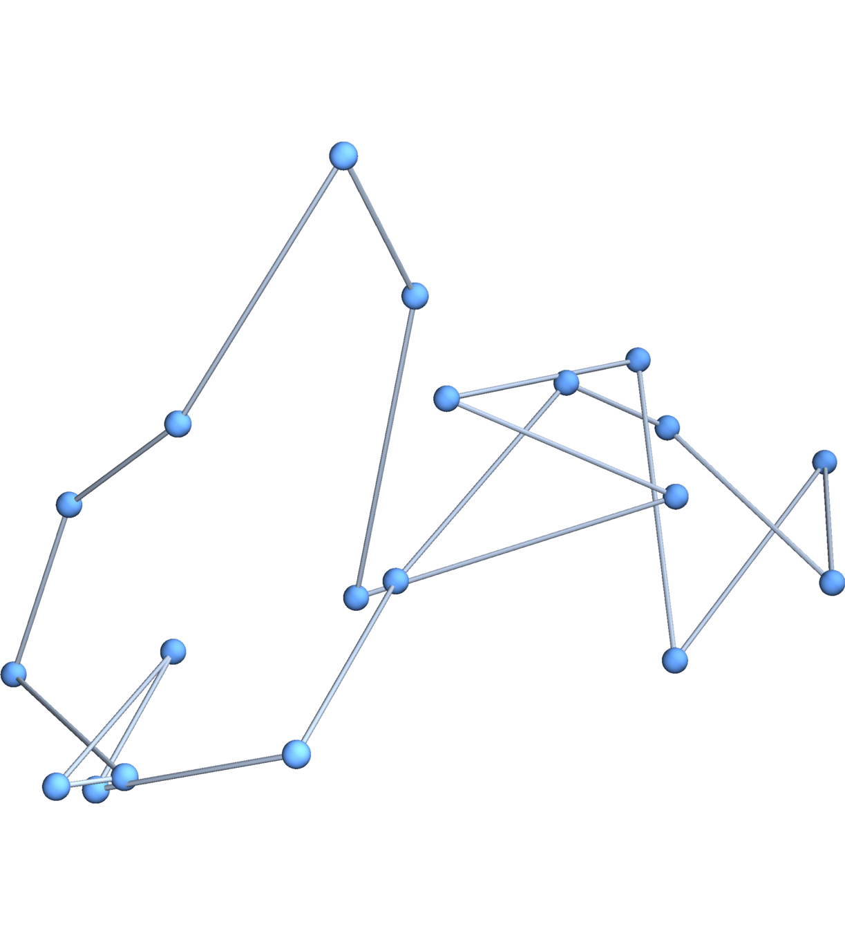
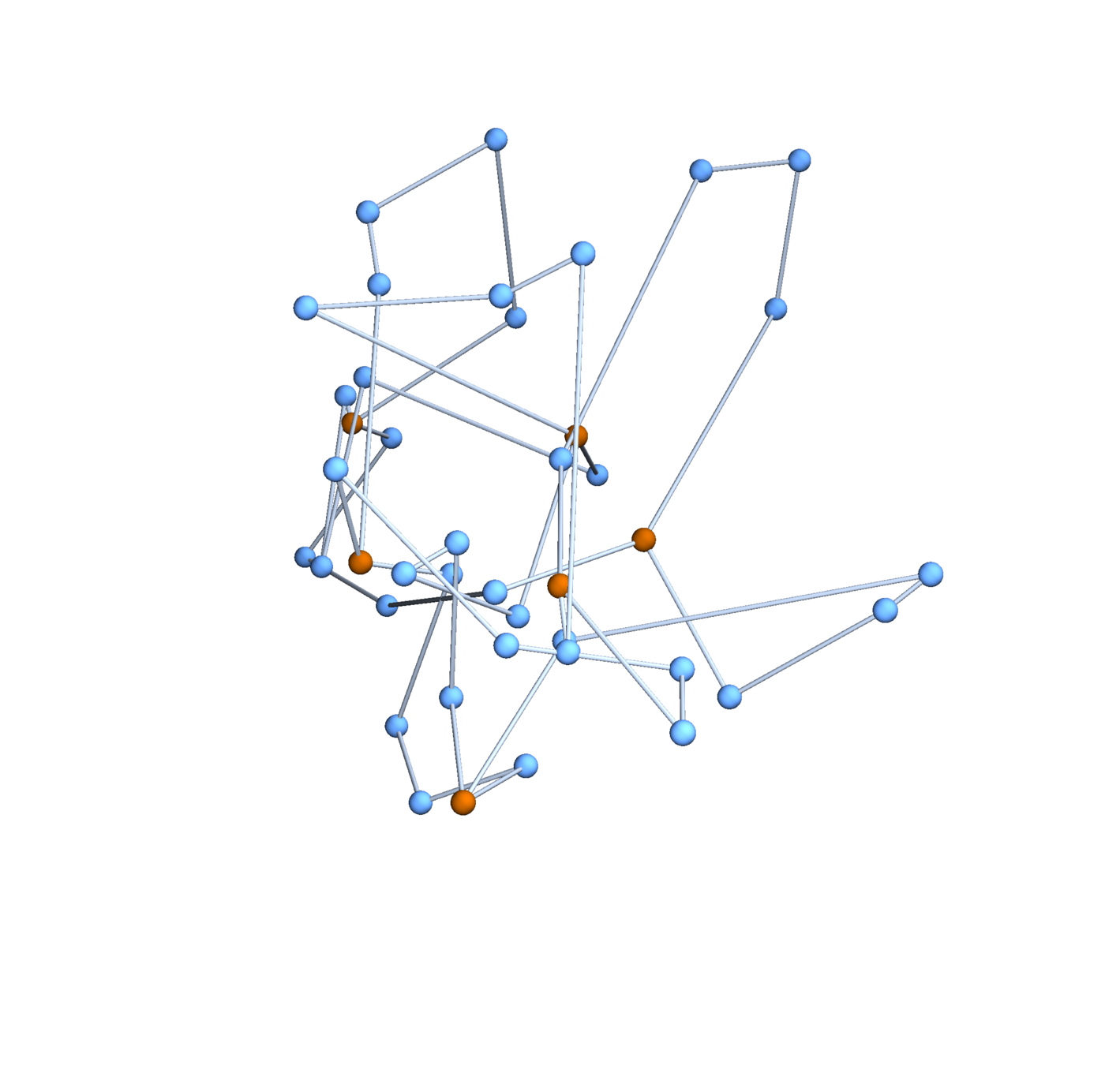
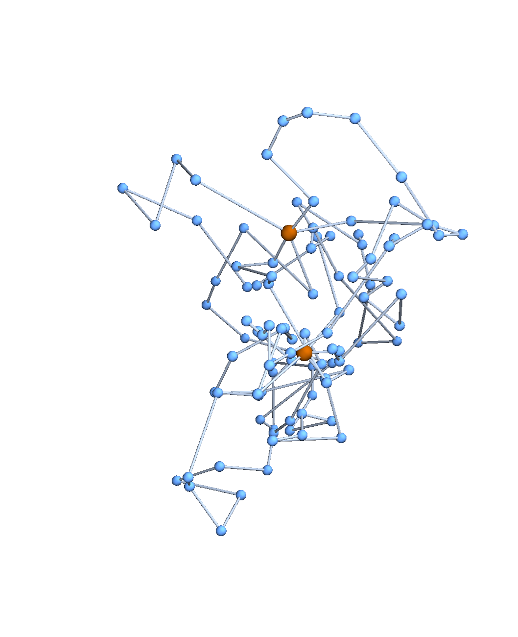
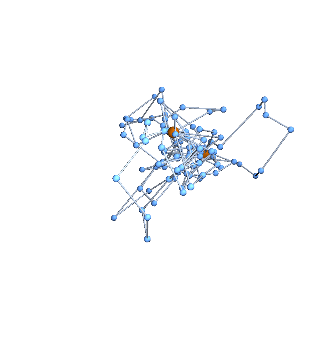
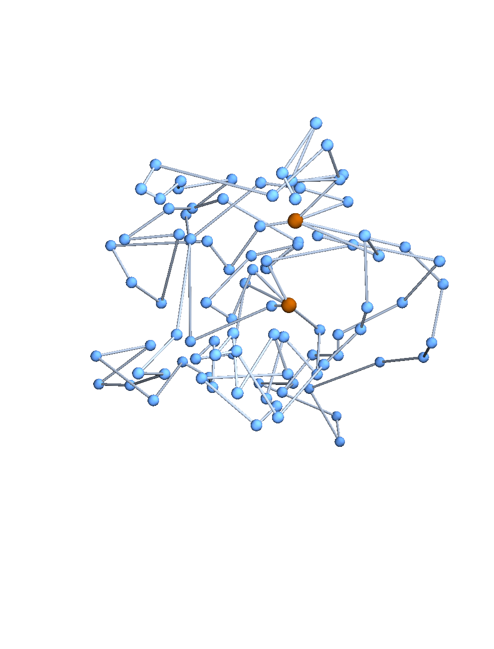
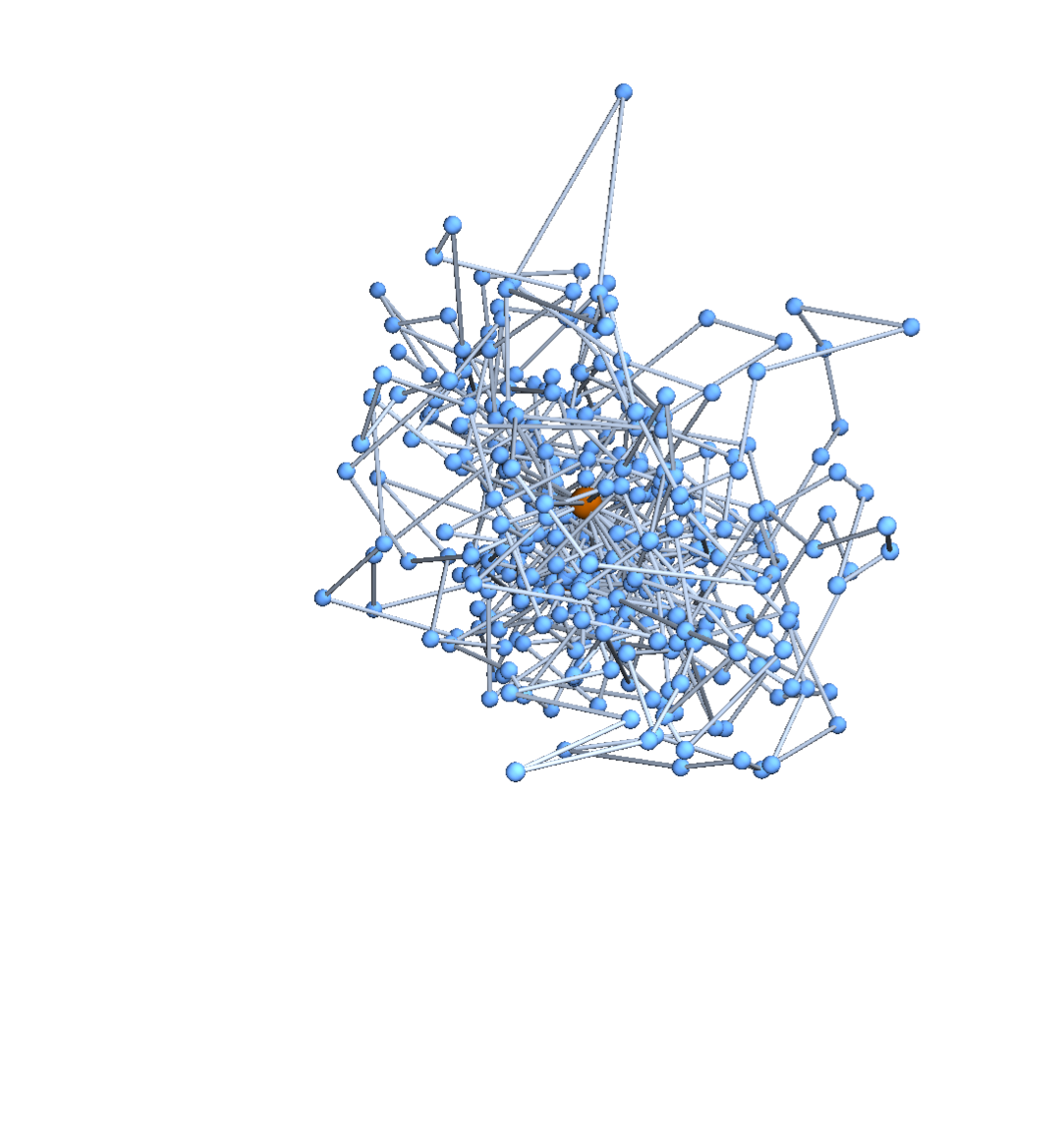
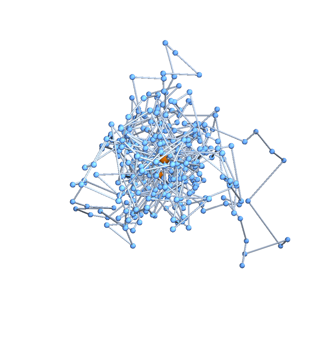
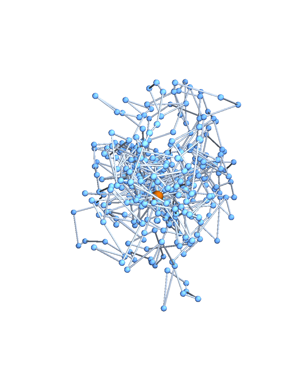
Gaussian embeddings
Definition.
A function \(f:\{v_i\} \to \mathbb{R}^d\) determines an embedding of \(\mathfrak{G}\) into \(\mathbb{R}^d\). The displacement vectors between adjacent vertices are given by \(\operatorname{grad}f\).
A Gaussian random embedding of \(\mathfrak{G}\) has displacements sampled from a standard multivariate Gaussian on \((\text{gradient fields})^d\subset \left(\mathbb{R}^\mathfrak{E}\right)^d\).
Useful lemma
Lemma. The projections of a Gaussian random embedding of \(\mathfrak{G}\) in \(\mathbb{R}^d\) onto each coordinate axis are independent Gaussian random embeddings of \(\mathfrak{G}\) into \(\mathbb{R}\).
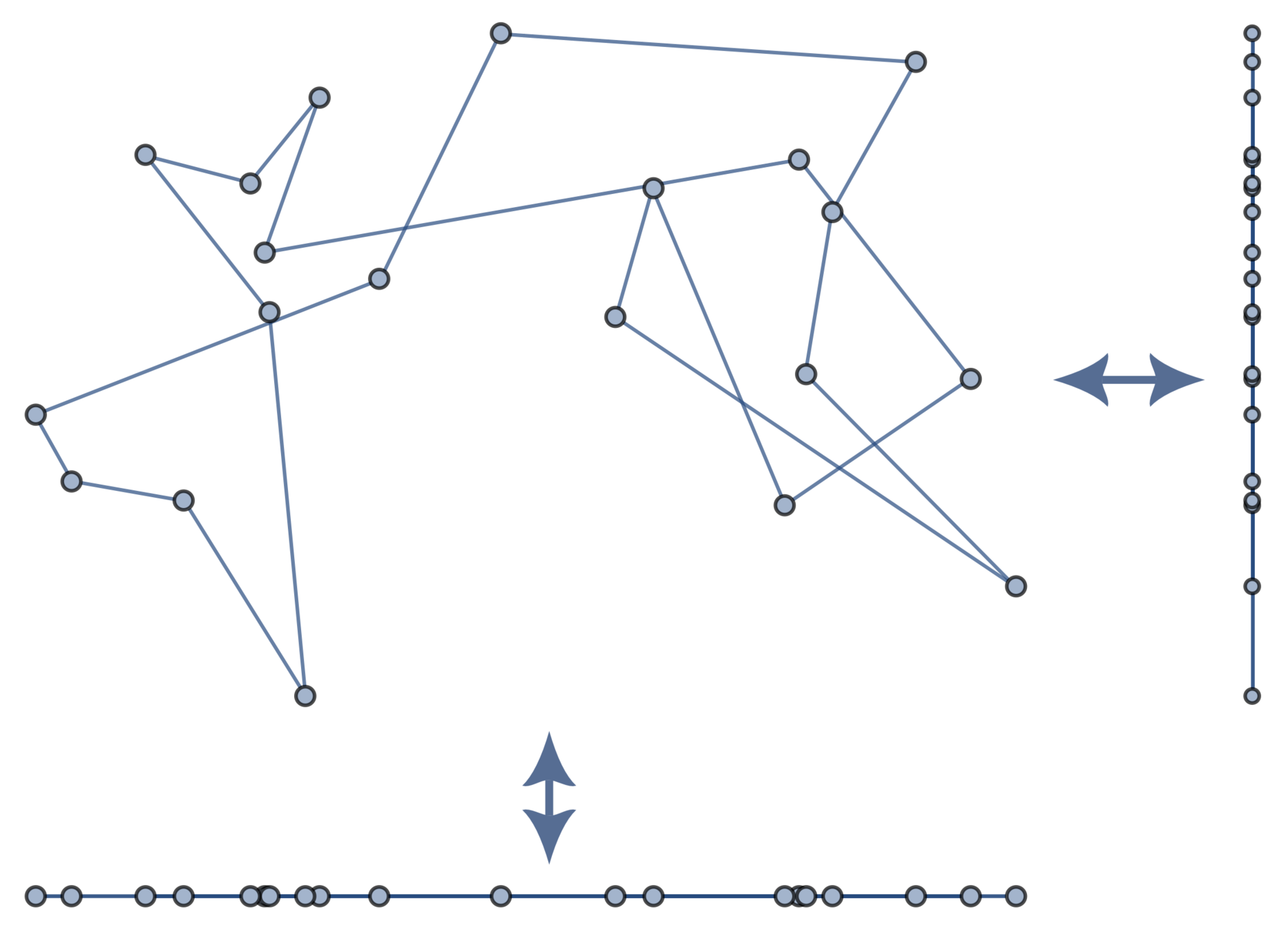
So we can restrict to Gaussian embeddings of \(\mathfrak{G}\) in \(\mathbb{R}\).
Main Theorem
Since \(\operatorname{grad}f=0 \,\Longleftrightarrow f\) is a constant function, \(\operatorname{grad}f\) only determines \(f\) up to a constant. So assume our random embeddings are centered; i.e., \(\sum f(v_i) = 0\).
Theorem [w/ CDU; cf. James, 1947]
The distribution of vertex positions on the \((\mathfrak{V}-1)\)-dimensional subspace of centered embeddings is
\(BB^T = \operatorname{div}\operatorname{grad} = L \) is the graph Laplacian
Pseudoinverse
For symmetric matrices like \(L \), with eigenvalues \(\lambda_i\) and eigenvectors \(v_i\), the pseudoinverse \(L^+\) is the symmetric matrix defined by:
- The eigenvalues \(\lambda_i'\) of \(L^+\) are
- The eigenvectors \(v_i'\) of \(L^+\) are \(v_i' = v_i\).
Sampling algorithm
Algorithm.
- Generate \(w\) from \(\mathcal{N}(0,I_\mathfrak{E})\)
- Let \(f = {B^T}^+ w\), which is \(\mathcal{N}(0,L^+)\)
Expected distances
Theorem [w/ CDU; cf. James, 1947]
The distribution of vertex positions on the \((\mathfrak{V}-1)\)-dimensional subspace of centered embeddings is
Corollary.
The expected squared distance between vertex \(i\) and vertex \(j\) is
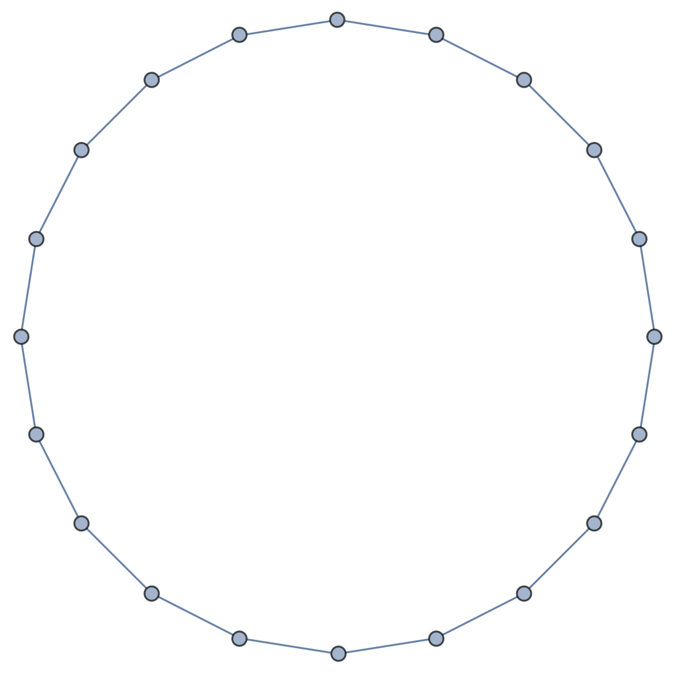
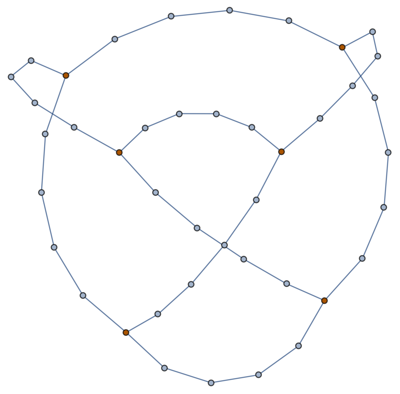
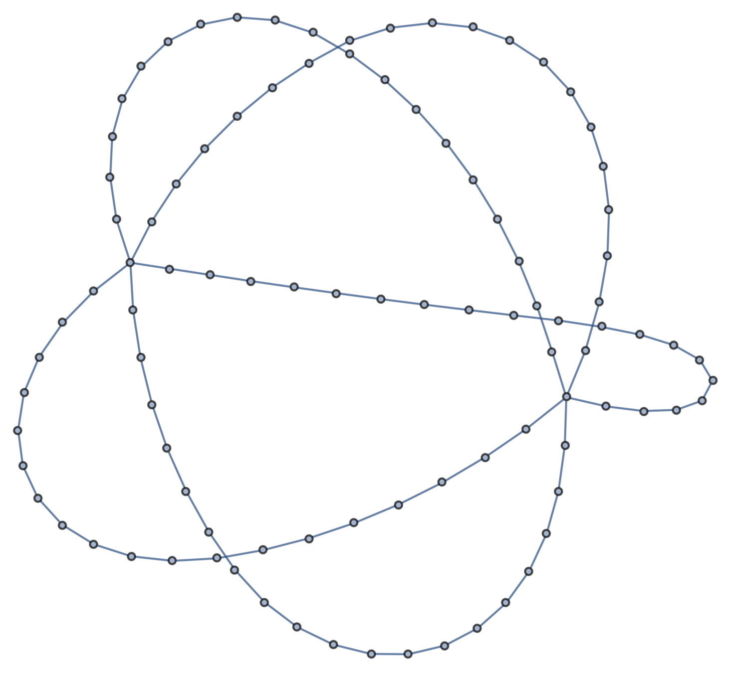
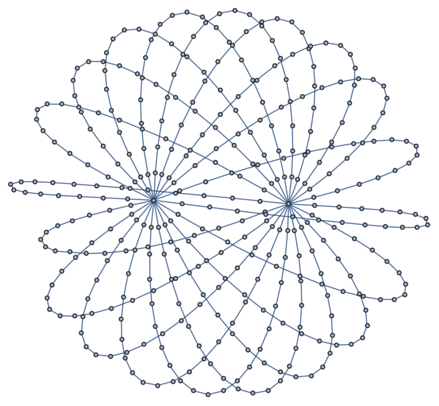
Example: multitheta graphs
Definition.
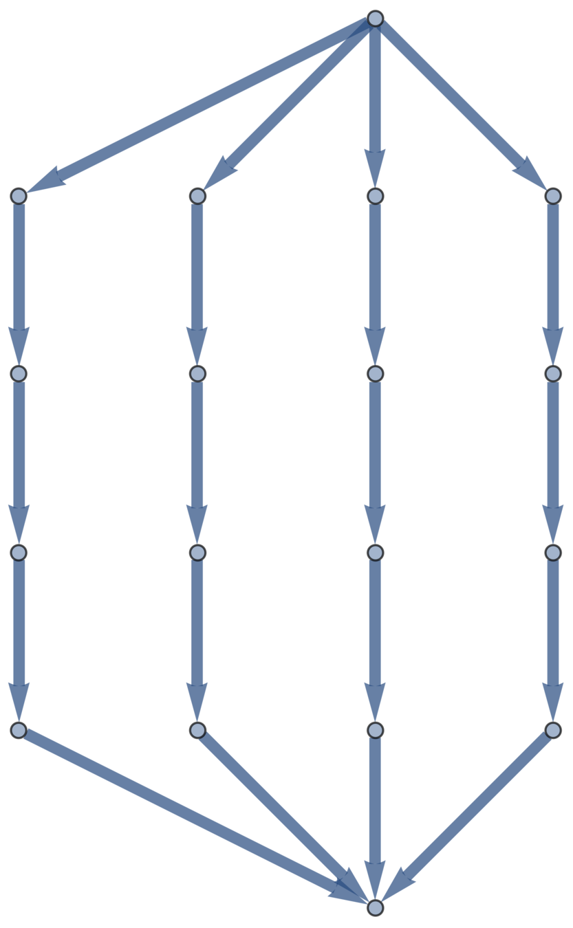
An \((m,n)\)-theta graph consists of \(m\) arcs of \(n\) edges connecting two junctions.
\((5,20)\)-theta graph
Theorem [Deguchi–Uehara, 2017]
The expected squared distance between junctions is \(\frac{dn}{m}\).
Amazing fact about \(L^+\)
Proposition [Nash–Williams (resistors, 1960s), James (springs, 1947)]
The expression \(L_{ii}^++L_{jj}^+-L_{ij}^+-L_{ji}^+\) is:
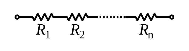
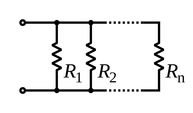
- the resistance between \(v_i\) and \(v_j\) if all edges of \(\mathfrak{G}\) are unit resistors;
- the reciprocal of the force between \(v_i\) and \(v_j\) if all edges are unit springs and \(v_i\) and \(v_j\) are one unit apart.
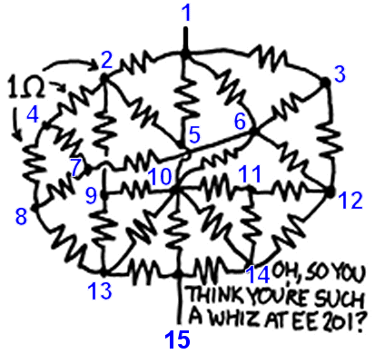
Randall Munro, [CC BY-NC 2.5], from xkcd
Deguchi–Uehara result, redux
Expected radius of gyration
Theorem [w/ CDU; cf. Estrada–Hatano, 2010]
If \(\lambda_i\) are the eigenvalues of \(L\), the expected squared radius of gyration of a Gaussian random embedding of \(\mathfrak{G}\) in \(\mathbb{R}^d\) is
This quantity is called the Kirchhoff index of \(\mathfrak{G}\).
Distinguishing graph types
Y. Tezuka, Acc. Chem. Res. 50 (2017), 2661–2672
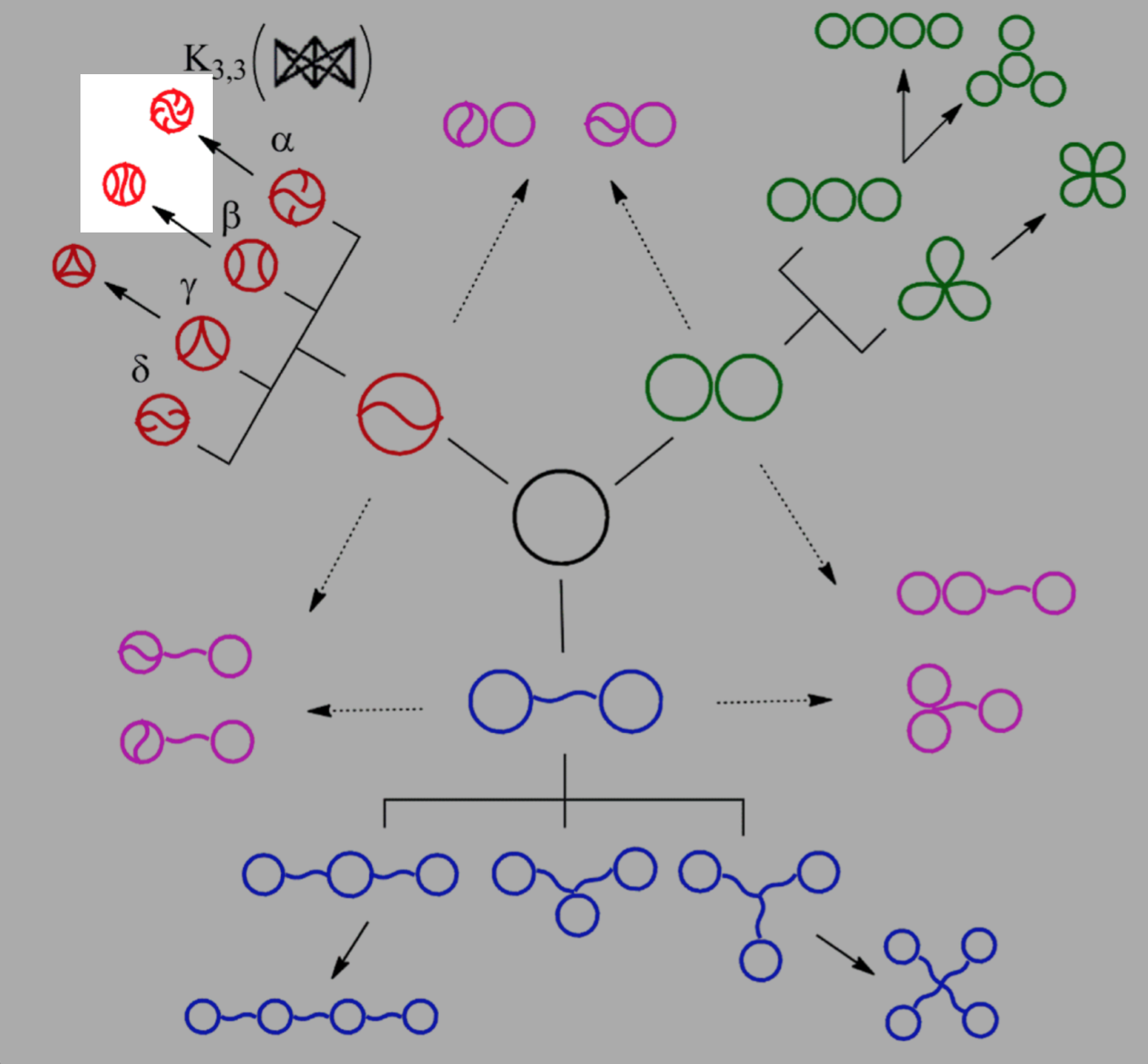
The suspects
T. Suzuki et al., J. Am. Chem. Soc. 136 (2014), 10148–10155
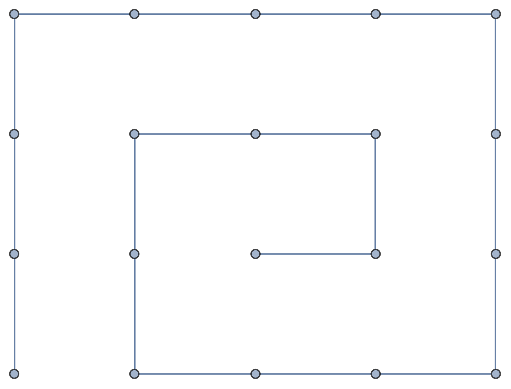
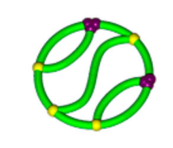
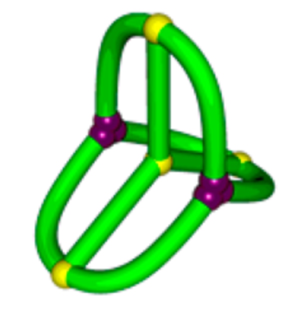
\(K_{3,3}\) (subdivided)
ladder graph (subdivided)
Topological polymers
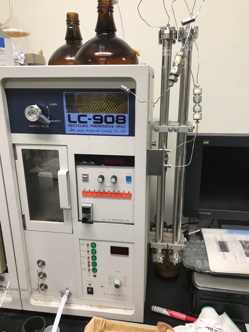
Size exclusion chromatograph
Distinguishing graph types in the lab
T. Suzuki et al., J. Am. Chem. Soc. 136 (2014), 10148–10155
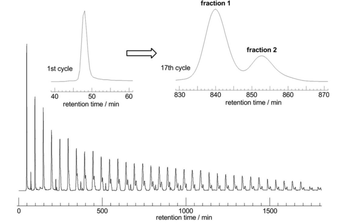
larger molecule
smaller molecule
Different sizes
Proposition [with Cantarella, Deguchi, & Uehara]
If each edge is subdivided equally to make \(\mathfrak{V}\) vertices total:
So the smaller molecule is predicted to be \(K_{3,3}\)!

Open questions
- Expectations are computable by computer algebra; are there analytic formulae for graph subdivisions?
- Topological type of graph embedding?
- What if the graph is a random graph?