Symplectic Geometry and Frame Theory
/mfo18
This talk!
Take Home Message
Symplectic geometry is a powerful set of tools which is useful for the study of frames
Frame Theory Basics
A frame in \(\mathbb{C}^k\) is a collection \(\{f_1,\dots ,f_N\}\subset \mathbb{C}^k\) so that
for some \(b\geq a > 0\) and for all \(v\in\mathbb{C}^k\).
The frame is tight if \(a=b\); equivalently, if \(F\) is the matrix with columns \(f_i\), then the frame operator \(FF^*=\frac{1}{a}I_k\).
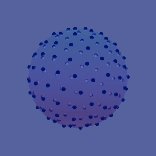
If \(\|f_i\|=1\) for all \(i\), the frame is unit norm. We abbreviate (Finite) Unit Norm Tight Frame as FUNTF.
Examples.
Notation
\(\mathcal{F}^{N,k}_S\) is the collection of length-\(N\) frames in \(\mathbb{C}^k\) with frame operator \(S\); i.e., \(k \times N\) matrices \(F\) with \(FF^*=S\).
Note that \(S\) is necessarily invertible and positive-definite.
\(\mathcal{F}^{N,k}_S(\vec{r})\) is the subset of \(\mathcal{F}^{N,k}_S\) of frames with \(\|f_i\| = r_i\).
In particular, the length-\(N\) FUNTFs in \(\mathbb{C}^k\) are precisely \(\mathcal{F}^{N,k}_{\frac{N}{k}I_k}(\vec{1})\) since
Symplecti-what?
Definition. A symplectic manifold is a smooth manifold \(M\) together with a closed, non-degenerate 2-form \({\omega \in \Omega^2(M)}\).
Example: \((S^2,d\theta\wedge dz)\)
Example. \((\mathbb{R}^2,dx \wedge dy) = (\mathbb{C},\frac{i}{2}dz \wedge d\bar{z})\)
Example. \((T^*\mathbb{R}^n, \sum_{i=1}^n dq_i \wedge dp_i)\)
Example. \((S^2,\omega)\), where \(\omega_p(u,v) = (u \times v) \cdot p\)
Example. \((\mathbb{R}^2,\omega)\) where \(\omega(u,v) = \langle i u, v \rangle \)
Example. \((\mathbb{C}^n, \frac{i}{2} \sum dz_k \wedge d\overline{z}_k)\)
Complex Geometry
If \((M,\omega)\) is symplectic and \(g\) is a Riemannian metric on \(M\), then \(g(\cdot, \cdot) = \omega(\cdot , J \cdot)\) defines a compatible almost complex structure \(J\) on \(M\).
If this compatible almost complex structure is integrable, then \((M,J,g,\omega)\) is Kähler.
Since the Fubini–Study form \(\omega_{\text{FS}}\) on \(\mathbb{CP}^n\) is Kähler, all smooth projective varieties are Kähler, and in particular symplectic.
The name ‘complex group’ formerly proposed by me..has become more and more embarrassing through collision with the word ‘complex’ in the connotation of complex number. I therefore propose to replace it by the corresponding Greek adjective ‘symplectic’.
— Hermann Weyl
Consequences
A symplectic manifold must be even-dimensional (over \(\mathbb{R}\)).
\(\omega^{\wedge n} = \omega \wedge \dots \wedge \omega\) is a volume form on \(M\), and induces a measure
called Liouville measure on \(M\).
If \(H: M \to \mathbb{R}\) is smooth, then there exists a unique vector field \(X_H\) (the Hamiltonian vector field for \(H\)) so that \({dH = \iota_{X_H}\omega}\), i.e.,
(\(X_H\) is sometimes called the symplectic gradient of \(H\))
Example
\(H: (S^2, d\theta\wedge dz) \to \mathbb{R}\) given by \(H(\theta,z) = z\).
\(dH = dz = \iota_{\frac{\partial}{\partial \theta}}\omega\), so \(X_H = \frac{\partial}{\partial \theta}\).
Integrating \(X_H\) produces the one-parameter family of diffeomorphisms \(\phi_t(\theta, z) = (\theta+t,z)\).
Lie Group Actions
Let \(G\) be a Lie group, and let \(\mathfrak{g}\) be its Lie algebra. If \(G\) acts on \((M,\omega)\), then each \(V \in \mathfrak{g}\) determines a vector field \(X_V\) on \(M\) by
\(S^1=U(1)\) acts on \((S^2,d\theta \wedge dz)\) by
For \(r \in \mathbb{R} \simeq \mathfrak{u}(1)\), \(X_r = r \frac{\partial}{\partial \theta}\).
Lie Group Actions
Let \(G\) be a Lie group, and let \(\mathfrak{g}\) be its Lie algebra. If \(G\) acts on \((M,\omega)\), then each \(V \in \mathfrak{g}\) determines a vector field \(X_V\) on \(M\) by
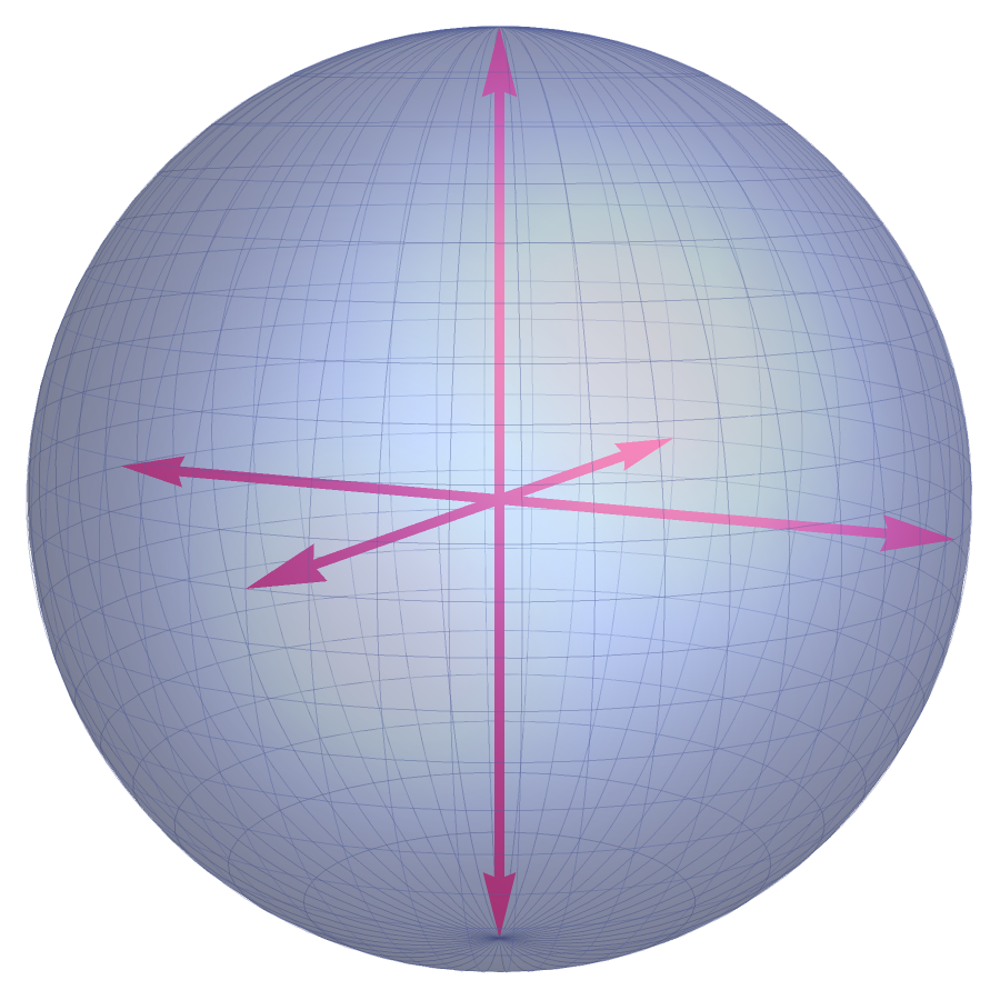
\(SO(3)\) acts on \(S^2\) by rotations.
\(X_{V_{(a,b,c)}}((x,y,z)) = (bz-cy)\frac{\partial}{\partial x} + (cx - az) \frac{\partial}{\partial y} + (ay - bx) \frac{\partial}{\partial z}\)
For \(V_{(a,b,c)} = \begin{bmatrix} 0 & -c & b \\ c & 0 & -a \\ -b & a & 0 \end{bmatrix} \in \mathfrak{so}(3)\),
\(= (a,b,c) \times (x,y,z)\)
Moment(um) Maps
Definition. An action of \(U(1)\) on \((M,\omega)\) is Hamiltonian if there exists a map
so that \(d\mu = \iota_{X}\omega\), where \(X\) is the vector field generated by the circle action.
\(X = \frac{\partial}{\partial \theta}\)
\(\iota_X\omega = \iota_{\frac{\partial}{\partial \theta}} d\theta \wedge dz = dz \)
\(\mu(\theta,z) = z\)
Moment(um) Maps
Definition. An action of \(G\) on \((M,\omega)\) is Hamiltonian if each one-parameter subgroup action is Hamiltonian. Equivalently, there exists a map
so that \(\omega_p(X_V, X) = D_p \mu(X)(V)\) for each \(p \in M\), \(X \in T_pM\), and \(V \in \mathfrak{g}\).
\(X_{V_{(a,b,c)}}(x,y,z) = (a,b,c) \times (x,y,z)\)
\((\iota_{X_{V_{(a,b,c)}}}\omega)_{(x,y,z)} = a dx + b dy + c dz \)
\(\mu(x,y,z)(V_{(a,b,c)}) = (x,y,z)\cdot(a,b,c)\)
A Circle Action on \(\mathbb{C}^k\)
Let \(U(1)\) act on \((\mathbb{C}^k,\omega_{\text{std}})\) by scalar multiplication.
The vector field generated by the circle action is
so \((\iota_X\omega_{\text{std}})_{\vec{v}}(Y) = (\omega_{\text{std}})_{\vec{v}}(X,Y) = \langle iX,Y\rangle_{\vec{v}} = \langle -\vec{v},Y\rangle\).
The moment map is
since \(d\mu_{\vec{v}}(Y) = \left.\frac{d}{dt}\right|_{t=0} \left(-\frac{1}{2} \langle \vec{v} + tY, \vec{v} + tY\rangle\right) = \langle -\vec{v},Y\rangle\).
The Big Guns
Theorem (Atiyah, Guillemin–Sternberg).
Let \((M^{2n},\omega)\) be a compact connected symplectic manifold with a Hamiltonian \(d\)-torus action with momentum map \(\mu: M \to \mathbb{R}^d\). Then
- the nonempty level sets of \(\mu\) are connected;
- the image of \(\mu\) is convex (called the moment polytope);
- the image of \(\mu\) is the convex hull of the images of fixed points of the action.
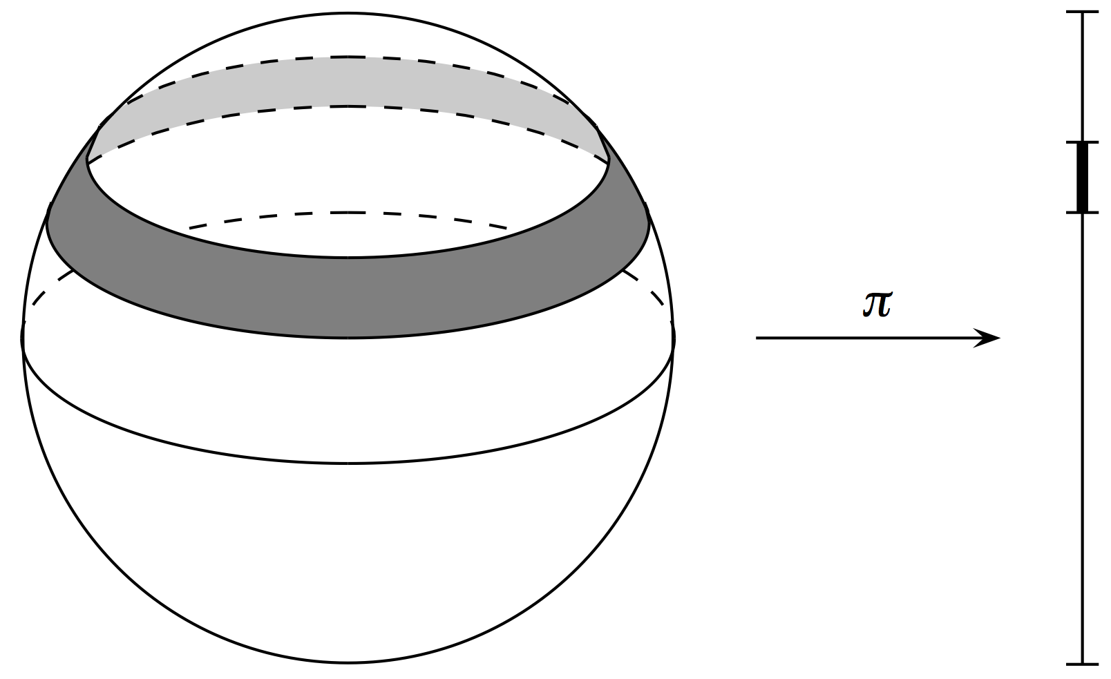
Theorem (Duistermaat–Heckman)
The pushforward of Liouville measure on \((M^{2n},\omega)\) to the moment polytope is absolutely continuous w.r.t. Lebesgue measure, with continuous, piecewise-polynomial density of degree \(\leq n-d\).
Example
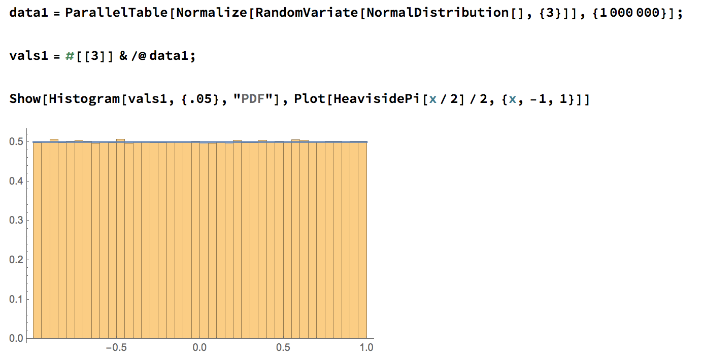
Theorem (Archimedes)
Let \(\mu: S^2 \to \mathbb{R}\) be given by \(\mu(x,y,z) = z\). Pushing forward the uniform measure on \(S^2\) to the image \([-1,1]\) gives Lebesgue measure.
Example 2
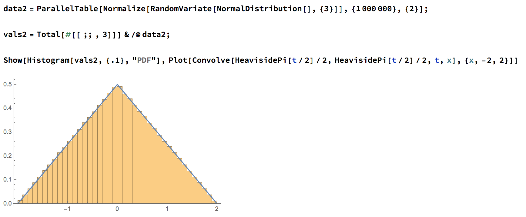
Proposition. If we rotate both factors of \(S^2 \times S^2\) simultaneously around the \(z\)-axis, the moment map is \(((x_1,y_1,z_1),(x_2,y_2,z_2))\mapsto z_1 + z_2\), and the pushforward measure on \([-2,2]\) has density given by the triangle function.
Complex Example
The \(\mathbb{T}^2 = U(1) \times U(1)\) action on \(\mathbb{CP}^2\) given by
has moment map
Symplectic Quotients
Theorem (Mayer, Marsden–Weinstein)
Let \(\mu: M \to \mathfrak{g}^*\) be the moment map for a Hamiltonian action of \(G\) on \((M,\omega)\). If \(\xi \in \mathfrak{g}^*\) is a regular value of \(\mu\) and \(\mathcal{O}_\xi\) is its coadjoint orbit, then
is a symplectic manifold with symplectic form \(\omega_{\text{red}}\) such that
\(\mu^{-1}(\mathcal{O}_\xi)\)
\(M /\!/\!_\xi\, G = \mu^{-1}(\mathcal{O}_\xi)/G\)
\(M\)
\(\pi\)
\(\iota\)
A Frame-Adjacent Example
\(U(1)^N\) acts on \(\mathbb{C}^{k \times N}\) by right-multiplication by diagonal unitary matrices.
Columnwise, this is the \(U(1)\) action on \(\mathbb{C}^k\) with moment map \(\vec{v} \mapsto -\frac{1}{2}|\vec{v}|^2\).
The moment map for the big torus action is
If \(-\vec{\frac{1}{2}} = \left(-\frac{1}{2},\dots , -\frac{1}{2}\right)\), then \(\widetilde{\Phi}^{-1}\!\left(-\vec{\frac{1}{2}}\right)\simeq \left(S^{2k-1}\right)^N\) consists of all matrices with unit-norm columns and
If \(\vec{w} \in \operatorname{image}(\widetilde{\Phi})\), then \(\widetilde{\Phi}^{-1}\!\left(\vec{w}\right)\simeq \prod_{i=1}^NS^{2k-1}(\sqrt{-2w_i})\) consists of matrices with column norms given by the \(\sqrt{-2w_i}\) and
A Frame-Related Example
\(U(k)\) acts on \(\mathbb{C}^{k \times N}\) by left multiplication with moment map
given by
Hermitian \(k \times k\) matrices
For invertible, positive-definite \(S \in \mathcal{H}(k)\), \(\mu^{-1}(S) = \mathcal{F}^{N,k}_S\), the set of frames with frame operator \(S\).
E.g., \(\mathcal{F}^{N,k}_{I_k}= \mu^{-1}(I_k)\) is (some of) the tight frames.
E.g., \(\mathcal{F}^{N,k}_{\frac{N}{k}I_k} = \mu^{-1}\left(\frac{N}{k}I_k\right)\) is (some of) the tight frames.
Grassmannians Enter the Story
Recall \(\mathcal{F}^{N,k}_{\frac{N}{k}I_k} = \left\{F : FF^* = \frac{N}{k}I_k\right\}\) is the space of tight frames which contains the FUNTFs.
is symplectic.
Observation.
...and Flag Manifolds
If \(S \in \mathcal{H}(k) \simeq \mathfrak{u}(k)^*\) is invertible and positive-definite, with eigenvalues \(\lambda_1 > \lambda_2 > \dots > \lambda_\ell > 0\) of multiplicities \(k_1, \dots , k_\ell\), then
where \(d_i = \sum_{j=1}^i k_j\).
is symplectic. \(\mu^{-1}(\mathcal{O}_S)\) is the space of all frames whose frame operator is conjugate to \(S\); call it \(\widetilde{\mathcal{F}^{N,k}_S}\).
FUNTFs
Notice that FUNTF space \(\mathcal{F}_{\frac{N}{k}I_k}(\vec{1})\) is exactly
The \(U(1)^N\) action on \(\mathbb{C}^{k \times N}\) induces an action on \(\operatorname{Gr}_k(\mathbb{C}^N)\); since the diagonal \(U(1)\) acts trivially, this is an effective \(U(1)^{N-1}\) action with moment map \(\Phi: \operatorname{Gr}_k(\mathbb{C}^N) \to \mathbb{R}^{N-1}\)
By Atiyah’s connectedness theorem, this is connected!
The Frame Homotopy Conjecture
Theorem (Cahill–Mixon–Strawn ’17)
The space \(\mathcal{F}^{N,k}_{\frac{N}{k}I_k}(\vec{1})\) of length-\(N\) FUNTFs in \(\mathbb{C}^k\) is path-connected for all \(N \geq k\geq 2\).
Proof. \(U(k) \backslash\mathcal{F}^{N,k}_{\frac{N}{k}I_k}(\vec{1}) = \Phi^{-1}\!\left(-\vec{\frac{1}{2}}\right)\) is connected.
Since \(U(k)\) is connected, the total space \(\mathcal{F}_{\frac{N}{k}I_k}(\vec{1})\) is connected.
Since this is a real algebraic set in \(\mathbb{C}^{k \times N} \simeq \mathbb{R}^{2kN}\), it is locally path-connected and therefore path-connected.
A Generalization
Theorem (with Needham ’18)
For any frame operator \(S\) and any admissible vector \(\vec{r}\) of frame norms, the space \(\mathcal{F}^{N,k}_S (\vec{r})\) is path-connected.
Proof idea.
is connected by Atiyah’s connectedness theorem, so \(\widetilde{\mathcal{F}^{N,k}_S}(\vec{r})\) is connected and path-connected.
If \(V_t\) is a path in \(\widetilde{\mathcal{F}^{N,k}_S}(\vec{r})\) connecting two points \({V_0,V_1 \in \mathcal{F}^{N,k}_S(\vec{r})}\), then \(V_tV_t^* = U_t^*SU_t\) and \(U_tV_t\) also connects \(V_0\) to \(V_1\) and stays in \(\mathcal{F}^{N,k}_S(\vec{r})\).
Questions
is (almost) toric, and in particular is measure-theoretically isomorphic to the product of the moment polytope (eigenstep polytope) and a torus. This should lead to a sampling algorithm for FUNTFs...
1.
2.
3.
Is there a corresponding story for frames on an infinite-dimensional Hilbert space?
What’s the version of the generalized frame homotopy theorem that applies to real frames? For example, \(\mathcal{F}^{6,\mathbb{R}^2}_{\frac{15}{2}I_2}(2,2,2,1,1,1)\) is not connected.
Thank you!
References
Symplectic geometry and connectivity of space of frames
Tom Needham and Clayton Shonkwiler
Funding: Simons Foundation
The geometry of constrained random walks and an application to frame theory
Clayton Shonkwiler
2018 IEEE Statistical Signal Processing Workshop (SSP), 343–347