Reading Group:

Efficient Neural Audio Synthesis

Computation Time

and

Call Overhead

T(\mathbf{u}) = |\mathbf{u}| \sum \Big( \text{comp}(\text{op}_i) + \text{call}(\text{op}_i) \Big)

T(\mathbf{u}) = |\mathbf{u}| \sum \Big( \text{comp}(\text{op}_i) + \text{call}(\text{op}_i) \Big)

T(u) = |u| \sum \Big( \text{c}(\text{op}_i) + \text{d}(\text{op}_i) \Big)

T(u) = |u| \sum \Big( \text{c}(\text{op}_i) + \text{d}(\text{op}_i) \Big)

where
comp is the computational overhead
(time spent MatMul'ing)
and
call is the call overhead
(i.e. how slow it is to launch a CUDA kernel)

Note: the paper used c and d ... which is silly ...

Minimizing call overhead

The LSTM equation has numerous examples of:

All of them have the same input. Thus we can instead run:

As each GPU operation costs 5 microseconds per call, we just saved 15 microseconds per timestep

GOOD WORK YOU! ^_^

W^i x_t, W^f x_t, W^o x_t, W^c x_t, \ldots

W^i x_t, W^f x_t, W^o x_t, W^c x_t, \ldots

[W^i, W^f, W^o, W^c] x_t

[W^i, W^f, W^o, W^c] x_t

Minimizing call overhead

We can doooooooooooo bettttttttttterrrrrrrrrrrr

Introducing the QRNN by Bradbury et al.

That entire concept is boiled down to:
The number of computations we do should be constant regardless of the number of timesteps

O(1) instead of O(n)

WaveRNN

In the input to WaveRNN, we have \(x_t = [c_{t-1}, f_{t-1}, c_t]\).
Wait ... How do we get \(c_t\) in \(x_t\)?

Let's look at the dependencies of each computation:
\(c_t\) relies on \(x_t = [c_{t-1}, f_{t-1}]\)
\(f_t\) relies on \(x_t = [c_{t-1}, f_{t-1}, c_t]\)

At training time,
Teacher force all \([c_{t-1}, f_{t-1}, c_t]\)

At test time,
First pass computes all for \(c_t\), most for \(f_t\)
Second pass only computes subset missing for \(f_t\)

WaveRNN

\(x_t = [c_{t-1}, f_{t-1}, c_t]\)

\(u_t = \sigma(R_u h_{t-1} + I_u^* x_t)\)

\(r_t = \sigma(R_r h_{t-1} + I_r^* x_t)\)

\(e_t = \tau(r_t \circ (R_e h_{t-1}) + I_e^* x_t)\)

\(h_t = u_t \circ h_{t-1} + (1 - u_t) \circ e_t\)

\(y_c, y_f = split(h_t)\)

\(P(c_t) = \text{softmax}(O_2 \text{relu}(O_1 y_c))\)

\(P(f_t) = \text{softmax}(O_4 \text{relu}(O_3 y_f))\)

WaveRNN

\(x_t = [c_{t-1}, f_{t-1}, c_t]\)

\(u_t = \sigma(R_u h_{t-1} + I_u^* x_t)\)

\(r_t = \sigma(R_r h_{t-1} + I_r^* x_t)\)

\(e_t = \tau(r_t \circ (R_e h_{t-1}) + I_e^* x_t)\)

\(h_t = u_t \circ h_{t-1} + (1 - u_t) \circ e_t\)

\(y_c, y_f = split(h_t)\)

\(P(c_t) = \text{softmax}(O_2 \text{relu}(O_1 y_c))\)

\(P(f_t) = \text{softmax}(O_4 \text{relu}(O_3 y_f))\)

GRU style candidate:

Reset gate:

Update gate:

Hidden update:

WaveRNN

\(x_t = [c_{t-1}, f_{t-1}, c_t]\)

\(u_t = \sigma(R_u h_{t-1} + I_u^* x_t)\)

\(r_t = \sigma(R_r h_{t-1} + I_r^* x_t)\)

\(e_t = \tau(r_t \circ (R_e h_{t-1}) + I_e^* x_t)\)

\(h_t = u_t \circ h_{t-1} + (1 - u_t) \circ e_t\)

GRU style candidate:

Reset gate:

Update gate:

Hidden update:

First run to get coarse \(c_t\),

then rerun for fine \(f_t\)

\(y_c, y_f = split(h_t)\)

\(P(c_t) = \text{softmax}(O_2 \text{relu}(O_1 y_c))\)

\(P(f_t) = \text{softmax}(O_4 \text{relu}(O_3 y_f))\)

WaveRNN

\(x_t = [c_{t-1}, f_{t-1}, c_t]\)

\(u_t = \sigma(R_u h_{t-1} + I_u^* x_t)\)

\(r_t = \sigma(R_r h_{t-1} + I_r^* x_t)\)

\(e_t = \tau(r_t \circ (R_e h_{t-1}) + I_e^* x_t)\)

\(h_t = u_t \circ h_{t-1} + (1 - u_t) \circ e_t\)

GRU style candidate:

Reset gate:

Update gate:

Hidden update:

First run to get coarse \(c_t\),

then rerun for fine \(f_t\)

\(y_c, y_f = split(h_t)\)

\(P(c_t) = \text{softmax}(O_2 \text{relu}(O_1 y_c))\)

\(P(f_t) = \text{softmax}(O_4 \text{relu}(O_3 y_f))\)

These matrix multiplications can be batched

WaveRNN

\(x_t = [c_{t-1}, f_{t-1}, c_t]\)

\(u_t = \sigma(R_u h_{t-1} + I_u^* x_t)\)

\(r_t = \sigma(R_r h_{t-1} + I_r^* x_t)\)

\(e_t = \tau(r_t \circ (R_e h_{t-1}) + I_e^* x_t)\)

\(h_t = u_t \circ h_{t-1} + (1 - u_t) \circ e_t\)

GRU style candidate:

Reset gate:

Update gate:

Hidden update:

First run to get coarse \(c_t\),

then rerun for fine \(f_t\)

\(y_c, y_f = split(h_t)\)

\(P(c_t) = \text{softmax}(O_2 \text{relu}(O_1 y_c))\)

\(P(f_t) = \text{softmax}(O_4 \text{relu}(O_3 y_f))\)

WaveNet: 60 matrix-vector products
WaveRNN: 5 matrix-vector products

Persistent RNNs

Every time you call a kernel, you need to reload the model's parameters - which is slow and redundant
Upper bound of 3x real time due to limited memory b/w

Persistent kernels load model params into register memory

NVIDIA P100 GPU has:
- 3.67M full precision registers
- Equal to over 7M half precision parameters
(see Baidu Persistent RNN, ...)

A single WaveRNN layer can happily squeeze into this space :)

Weight Sparsification

If we want to achieve a set sparsity (i.e. Z = 0.96),
every N steps we zero out the smallest k weights,
with k slowly increasing towards the desired sparsity

To encode the sparsity pattern naively is space intense - instead opt for a block based approach.

The cost of computing and storing is proportional to the number of non-zero parameters.

Weight Sparsification

The cost of computing and storing is proportional to the number of non-zero parameters.

For a fixed parameter count, large sparse models generally outperform small dense models.
Sparse models also play a role in space efficiency (mobile).

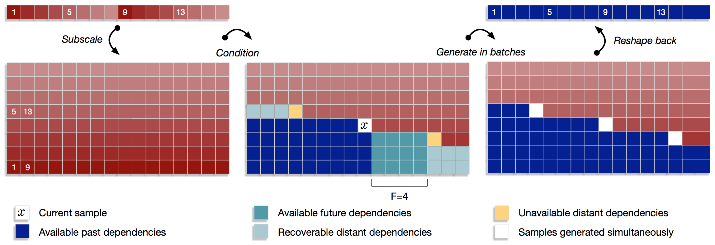
Subscale WaveRNN

Idea: Produce \(B\) samples per timestep rather than 1
(essentially allowed you to batch compute a single example)

This reduces the problem from \(|\mathbf{u}|\) to \(\frac{|\mathbf{u}|}{B}\)

This works well as:
- The GPU is rarely running at full capacity for small batch
- Weights + operations are re-used across the computations
- Audio has less strong "sharp" dependencies, esp locally

T(\mathbf{u}) = \frac{|\mathbf{u}|}{B} \sum \Big( \text{comp}(\text{op}_i) + \text{call}(\text{op}_i) \Big)

T(\mathbf{u}) = \frac{|\mathbf{u}|}{B} \sum \Big( \text{comp}(\text{op}_i) + \text{call}(\text{op}_i) \Big)

Subscale WaveRNN

This looks scary - and is a little - but we'll get through it!

...Maybe...

Subscale WaveRNN

This \(x_t\) has access to:
- 3 directly previous samples

Subscale WaveRNN

This \(x_t\) has access to:
- 3 directly previous samples
- 8 samples into the past spaced \(B\) apart

Subscale WaveRNN

This \(x_t\) has access to:
- 3 directly previous samples
- 8 samples into the past spaced \(B\) apart

- Many samples in the past (part complete sub-tensors)

Subscale WaveRNN

This \(x_t\) has access to:
- 3 directly previous samples
- 8 samples into the past spaced \(B\) apart

- Many samples in the past (part complete sub-tensors)

- Some samples in the future (up to \(F\) away)

Subscale WaveRNN

This \(x_t\) has access to:
- 3 directly previous samples
- 8 samples into the past spaced \(B\) apart

- Many samples in the past (part complete sub-tensors)

- Some samples in the future (up to \(F\) away)

- Optionally could condition on additional future samples

Subscale WaveRNN

This \(x_t\) has access to:
- 3 directly previous samples
- 8 samples into the past spaced \(B\) apart

- Many samples in the past (part complete sub-tensors)

- Some samples in the future (up to \(F\) away)

- Optionally could condition on additional future samples

Subscale WaveRNN

Thus multiple samples can be produced simultaneously -
by deciding we don't need exact history, just representative

Summary

Remember we can cheat with teacher forcing!

Ponder on bottlenecks and how existing models fail

"Roofline" your models - work out the maximum capabilities of your device and then see if you can take advantage of that

Large and sparse better than small and dense
(if you have crazy CUDA level optimization knowledge)

Sparsification allows for efficiency in storage and compute
(positively impacting from GPUs down to mobile CPUs)

We can generally achieve strong results by removing bad assumptions