Embed

Computational Biology

(BIOSC 1540)

Feb 25, 2025

Lecture 08A

Differential gene expression

Foundations

Announcements

César optional Python recitations are on Fridays from 2 - 3 pm in L1 Clapp Hall
Please fill out the Canvas discussion for CBit 07

Quiz 03 is on Mar 18 and will cover L06B to L08B

Assignments

P02A is due Mar 14
P02B will be published sometime this week

Quizzes

CBits

After today, you should have a better understanding of

Hypothesis testing for comparing gene expression

Let's remember the big picture: We want to quantify differences in gene expression

Differential gene expression quantifies changes in gene expression levels between different sample groups or conditions

We have been focused on quantifying gene expression in quantities like Transcripts Per Million (TPM)

Samples

Normal

Cancerous

We cannot rely on simple comparisons when analyzing gene expression

We could technically directly compare means between our different conditions

However, biological data are inherently noisy, and observed differences may arise by chance

Examples of experimental biases (besides sample variation)

Sequencing depth: Higher depth could appear as higher expression levels simply due to having more data

Batch effects: Processing sampling with different equipment, reagents, times, etc. can show systematic differences

Normal

Cancerous

TPM

Samples

We need approaches that address these sources of variation and noise

Normal

Cancerous

TPM

Samples

Statistical models can account for variability and separate signal from noise

Hypothesis testing between statistical models provides a quantitative way to compare conditions

Hypothesis testing in RNA-seq data

After fitting a statistical model, we need to perform hypothesis testing to see if the difference in expression between conditions is statistically significant

Gene expression

Normal

Cancerous

We reject the null hypothesis when our statistical test demonstrates that the observed difference, if any, is unlikely to have happened by random chance

Null Hypothesis (H₀): There is no difference in gene expression between the two conditions

Alternative Hypothesis (H₁): There is a significant difference in gene expression between the conditions

We have two hypotheses:

The p-value is the probability of the null hypothesis being true

What is the probability that any difference is either (1) nonexistent or (2) due to random chance

Probability value (p-value):

The higher the p-value, the more our model supports the null hypothesis

The lower the p-value, the more our model supports the alternative hypothesis

Gene expression

Normal

Cancerous

p \approx 0.9999

Gene expression

Normal

Cancerous

p \approx 0.00001

After today, you should have a better understanding of

Reliable statistical models for gene expression data

Binomial distribution

To compute probabilities under H₀, we need a model that describes expected variation

A statistical model describes how data is expected to behave if H₀ is true.

For example, a fair coin flip should result in a normal distribution centered on 50% of each side

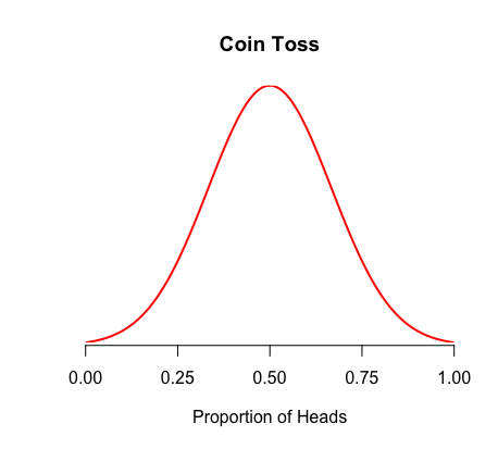
This is our statistical model that describes our coin flip observations under H₀

We are probably flipping a weighted coin because our observations do not match our H₀ statistical model

If we flip a coin 10 million times and our distribution looks like

this

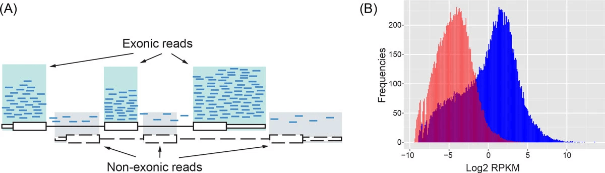
Gene expression data have unique challenges that require specific statistical models

The nature of count data

RNA-seq generates count data – the number of RNA fragments that map to each gene

Gene expression

Normal

Cancerous

Example: 573,282 TPM

Discrete data requires us to use special statistical models

Data that can only take whole numbers
In RNA-seq, we measure the number of transcripts, so the data are count-based
For example, you cannot have "half a transcript"

What is discrete data?

Binomial: A Simple Model for Discrete Counts

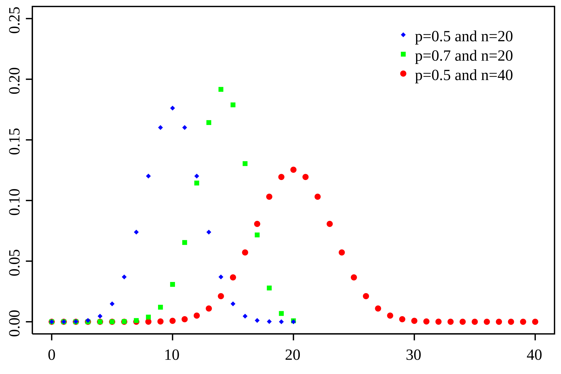
The Binomial distribution models the number of successes in a fixed number of independent trials, where each trial has the same probability of success

n

k

P

p

P \left( X = k \right) = \frac{n!}{k! \left( n - k \right)!} p^k \left( 1 - p \right)^{n - k}

Number of trials

Number of successes

Probability

Probability of success

RNA-seq analogy: Each read can be considered a "trial," and the probability that a read maps to a specific gene is the "probability of success."

k

P

After today, you should have a better understanding of

Reliable statistical models for gene expression data

Poisson distribution

Challenge #1: The binomial distribution assumes that the probability of success (p) is the same for every trial

For example, if I have 10 samples from cancerous cells, the binomial distribution assumes they are perfect replicates with no biases

Ignoring sample-to-sample variability can lead to underestimating the true uncertainty in the data

n

k

P

p

P \left( X = k \right) = \frac{n!}{k! \left( n - k \right)!} p^k \left( 1 - p \right)^{n - k}

Number of trials

Number of successes

Probability

Probability of success

Challenge #2: High sequencing depth results in an extremely large number of trials, posing both computational and modeling challenges

When sequencing depth is high, n (the total number of reads) becomes very large

Factorials when n is large makes accurate calculations impractical

P \left( X = k \right) = \frac{n!}{k! \left( n - k \right)!} p^k \left( 1 - p \right)^{n - k}

Challenge #3: For many genes, the probability of expression (p) is extremely low, further complicating the use of the binomial distribution

With very low p, the expected number of successes (reads mapping to a lowly expressed gene) is minuscule compared to n

P \left( X = k \right) = \frac{n!}{k! \left( n - k \right)!} p^k \left( 1 - p \right)^{n - k}

Calculations with very small probabilities may lead to numerical underflow/imprecise results

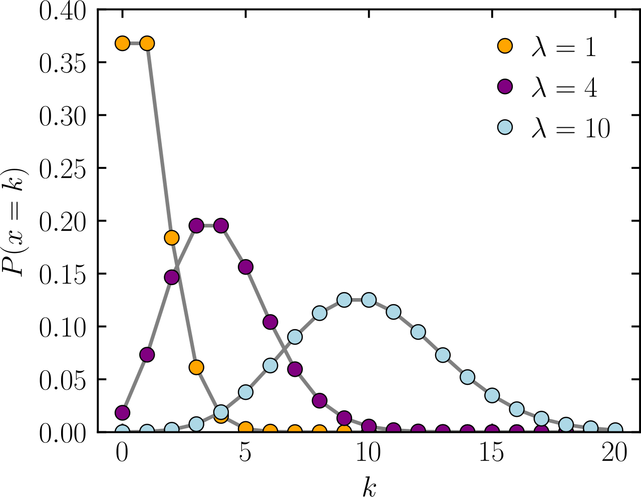
Poisson distribution: A tractable model for large discrete counts

The Poisson distribution is a statistical tool used to model the number of events (i.e., counts) that happen in a fixed period of time or space, where:

The events are independent of each other
Each event has a constant average rate (i.e., allows variation between events)

P \left( X = k \right) = \frac{\lambda^k e^{-\lambda}}{k!}

\lambda

Expected average of X

k

Number of events or counts

P

Probability

Assuming the constant average rate of success allows some variation around the mean

I.e., sample variation and batch effects

After today, you should have a better understanding of

Reliable statistical models for gene expression data

Negative binomial distribution

Poisson distribution assumes mean and variance are equal

E[X] = \sum_{k=0}^{\infty} k \cdot P(X = k) \\

The expected value (i.e., mean)

When k = 0, the term is zero

= \sum_{k=1}^{\infty} k \frac{\lambda^k e^{-\lambda}}{k!}

= \lambda e^{-\lambda} \sum_{k=1}^{\infty} \frac{\lambda^{k-1}}{(k-1)!}

k \frac{\lambda^k}{k!} = \lambda \frac{\lambda^{k-1}}{(k-1)!}

= \lambda e^{-\lambda} \sum_{j=0}^{\infty} \frac{\lambda^j}{j!}

j = k-1

Use

= \lambda e^{-\lambda} \cdot e^{\lambda} = \lambda

\sum_{j=0}^{\infty} \frac{\lambda^j}{j!} = e^{\lambda}

You don't need to understand these derivations—just the outcome

= \lambda

Poisson distribution assumes mean and variance are equal

Var(X) = E[X^2] - \left(E[X]\right)^2

E[X(X-1)] = \sum_{k=2}^{\infty} k(k-1) \frac{\lambda^k e^{-\lambda}}{k!}

E[X^2] = E[X(X-1)] + E[X]

When k = 0 or 1, the term is zero

k(k-1) \frac{\lambda^k}{k!} = \frac{\lambda^k}{(k-2)!}

= \sum_{k=2}^{\infty} k(k-1) \frac{\lambda^k e^{-\lambda}}{k!}

You don't need to understand these derivations—just the outcome

= e^{-\lambda} \sum_{k=2}^{\infty} \frac{\lambda^k}{(k-2)!}

= \lambda^2 e^{-\lambda} \sum_{j=0}^{\infty} \frac{\lambda^j}{j!}

j = k-2

Use

= \lambda^2 e^{-\lambda} \cdot e^{\lambda}

\sum_{j=0}^{\infty} \frac{\lambda^j}{j!} = e^{\lambda}

= (\lambda^2 + \lambda) - \lambda^2

=\lambda

E[X] = Var(X) = \lambda

= \lambda^2

If our variance is different from our mean, our Poisson model breaks down

Parity plots with mean and variance show deviations with Poisson distributions

Higher counts typically have a larger variance

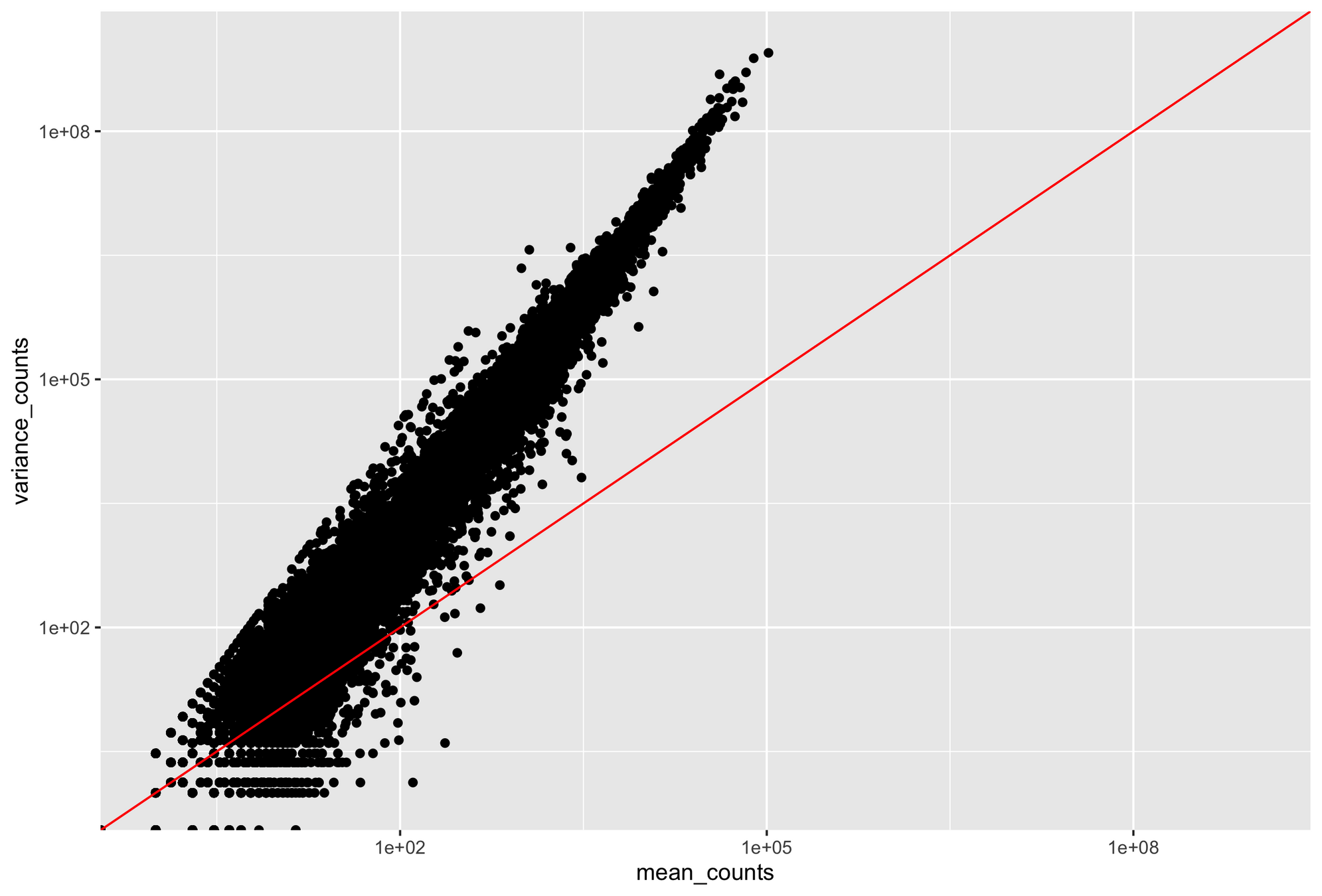
Count mean

Count variance

Mean = variance line

Overdispersion in RNA-Seq

Overdispersion: It happens when the variance in the data is larger than what is predicted by simpler models (e.g., Poisson distribution)

Expected variance for Poisson-distributed data equals the mean: $Variance=μ\text{Variance} = \mu$
Variance is often larger than the mean for RNA-Seq: $Variance>μ\text{Variance} > \mu$

Overdispersion may reflect biological variability between samples not captured by the experimental conditions

Differences in RNA quality
sequencing depth,
biological factors like different cell types within the same tissue

Poisson distribution is unsuitable for RNA-seq data because of high noise

Negative Binomial distribution accounts for high dispersion

P(X = k) = \frac{\Gamma(k + \frac{1}{\alpha})}{k! \, \Gamma(\frac{1}{\alpha})} \left(\frac{1}{1 + \alpha \mu}\right)^{\frac{1}{\alpha}} \left(\frac{\alpha \mu}{1 + \alpha \mu}\right)^k

k

Observed number of counts

\mu

Mean or expected value of counts

\alpha

Dispersion parameter, controlling how much the variance exceeds the mean

\Gamma \left( \cdot \right)

Gamma function, which generalizes the factorial to floats

\text{Var}(X) = \mu + \alpha \mu^2

If $α=0\alpha = 0$ , the Negative Binomial distribution reduces to the Poisson distribution

The challenge of zeros in RNA-seq data

RNA-seq data frequently contains zero counts for some genes because not all genes are expressed under all conditions

Most statistical models account for variance, but not that zeros can dominate counts

For example, if we have a high expected mean with Poisson distribution we can still have zeros or very low counts

In these circumstances, we have to use zero-inflated models

We will ignore these for now

After today, you should have a better understanding of

Fitting statistical models

Likelihood quantifies the probability of the observed data given a model

A higher product (or joint likelihood) means the model assigns a higher probability to the observed data, indicating a better fit.

The likelihood of model parameters $θ\theta$ given data $y\mathbf{y}$ is defined as

P(y_1, y_2, \ldots, y_n | \theta) = \prod_{i=1}^n P(y_i | \theta)

L(\theta) = P(\mathbf{y} | \theta)

When individual data points $y1,y2,…,yny_1, y_2, \dots, y_n$ are independent, the joint probability is calculated by multiplying their individual probabilities:

Multiplying these probabilities aggregates the evidence from each data point, providing a comprehensive measure of how well the model with parameter $θ\theta$ fits all the data

The log transformation simplifies computation and interpretation

$log⁡L(θ)=∑i=1nlog⁡P(yi∣θ)\log L(\theta) = \sum_{i=1}^n \log P(y_i|\theta)$

Makes differentiation easier for optimization

\log L(\theta) = \sum_{i=1}^n \log P(y_i|\theta)

Log likelihood

$log⁡L(θ)=∑i=1nlog⁡P(yi∣θ)\log L(\theta) = \sum_{i=1}^n \log P(y_i|\theta)$

Converts products into sums, reducing computational issues.

Maximum Likelihood Estimation (MLE) finds the parameters that maximize the log likelihood

At the optimum, the model parameters provide the best explanation of the observed data.

\hat{\theta} = \arg\max_{\theta} \log L(\theta)

Optimization problem

Bad fit

Good fit

After today, you should have a better understanding of

Statistical tests

Likelihood Ratio Test

To compute a p-value, a likelihood ratio test (LRT) can be used $β^1\hat{\beta}_1$

The idea is to compare the likelihood of the data under

the null model (same expression in both conditions)
the alternative model (different expression levels in each condition) $β^1\hat{\beta}_1$

Log-Likelihood of Negative Binomial

\log \mathcal{L}(r, \mu | X) = X \log \left( \frac{\mu}{\mu + r} \right) + r \log \left( \frac{r}{\mu + r} \right)

For each condition, you compute the log-likelihoods:

\mathcal{L}_{\text{A}} = \sum_{i} \log \mathcal{L}(r_A, \mu_A | X_i)

\mathcal{L}_{\text{B}} = \sum_{i} \log \mathcal{L}(r_B, \mu_B | X_i)

LRT Statistic

The LRT statistic is: $β^1\hat{\beta}_1$

\text{LRT} = -2 \left( \log \mathcal{L}_{\text{null}} - \left( \log \mathcal{L}_{\text{A}} + \log \mathcal{L}_{\text{B}} \right) \right)

\log \mathcal{L}_{\text{null}} = \sum_{i} \log \mathcal{L}(r_0, \mu_0 | X_i)

The log-likelihood under the null hypothesis (assuming a common mean $μ0\mu_0$ for both conditions)

The LRT statistic approximately follows a chi-squared distribution with 1 degree of freedom under the null hypothesis

The p-value is computed as:

p = 1 - F_{\chi^2_1}(\text{LRT})

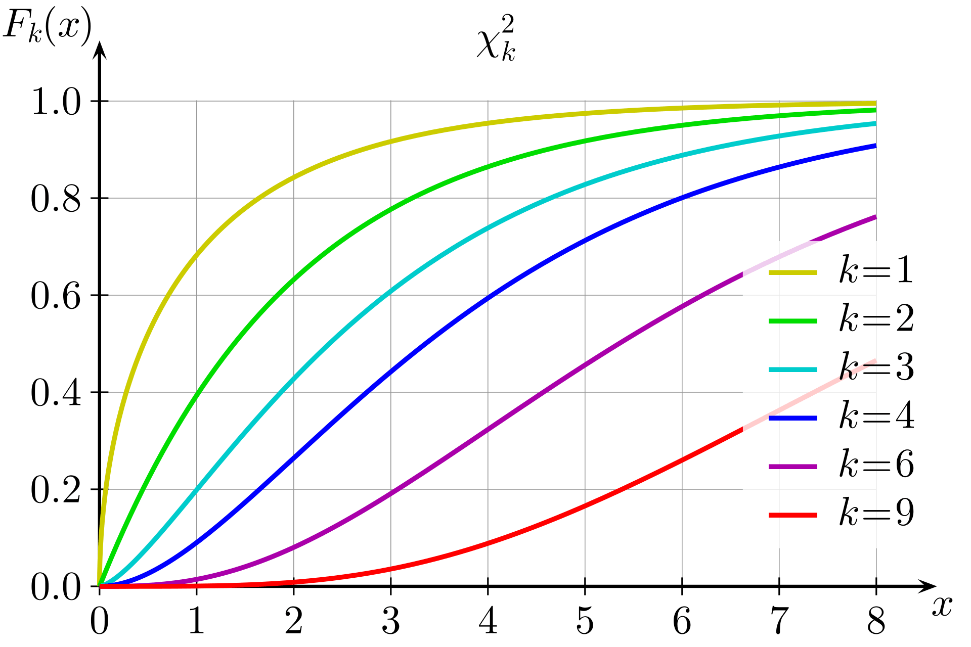
k would be 1

Example: Triple-negative breast breast cancer

Objective: Identify genes differentially expressed between triple-negative breast cancer (TNBC) and hormone receptor-positive breast cancer

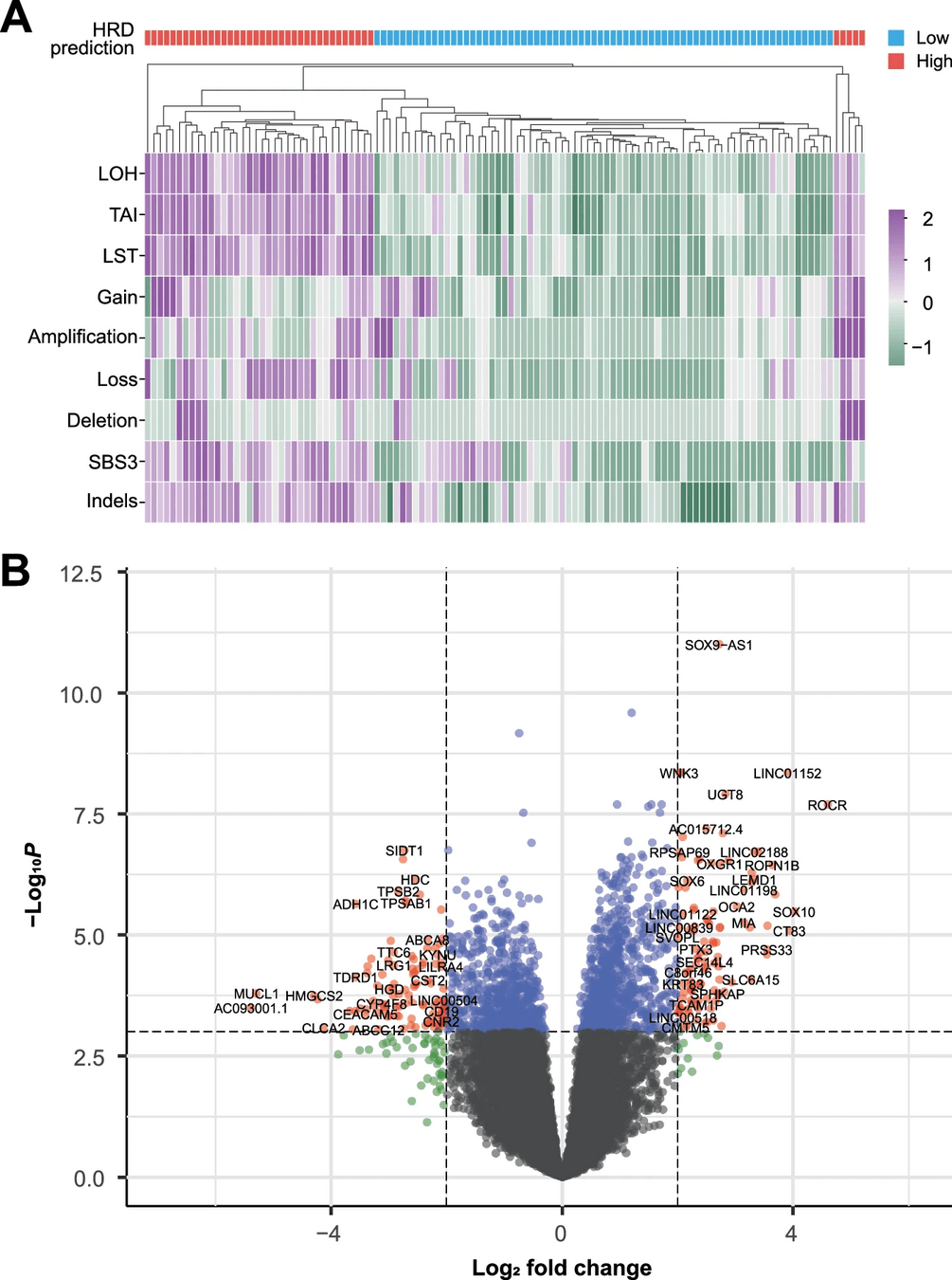
Differential gene expression provides statistical tools to identify changes between samples

Findings: TNBC shows upregulation of genes involved in cell proliferation and metastasis.

Implications:

Targets for specific therapies.
Improved classification and prognosis of breast cancer subtypes.

Wald’s Test for Gene Expression Differences

Wald’s Test: A statistical test that helps us determine whether the estimated log fold change between two conditions is significantly different from zero.
Null Hypothesis (H₀): The log fold change between conditions is zero (no difference in expression between the conditions).
- Log Fold Change (β₁) = 0 means that the gene is expressed at the same level in both conditions.
Alternative Hypothesis (H₁): The log fold change between conditions is not zero (there is a difference in expression).

Estimate Parameters from the Negative Binomial Model

For each gene, the Negative Binomial model gives us an estimated log fold change $β^1\hat{\beta}_1$

\hat{\beta}_1

It also gives us a standard error (SE) for this estimate, which tells us how uncertain we are about the estimate of log fold change $β^1\hat{\beta}_$

SE \left( \hat{\beta}_1 \right)

The Wald statistic is calculated as

\text{Wald statistic} = \frac{\hat{\beta}_1}{SE \left( \hat{\beta}_1 \right)}

This statistic tells us how many standard deviations the estimated log fold change is away from zero (no difference)

Log Fold Change

Positive Log Fold Change: Indicates higher expression in the condition of interest (e.g., diseased).
Negative Log Fold Change: Indicates lower expression in the condition of interest.
Log Fold Change of Zero: Means no difference between conditions.

Announcements

After today, you should have a better understanding of

Hypothesis testing for comparing gene expression

Let's remember the big picture: We want to quantify differences in gene expression

We cannot rely on simple comparisons when analyzing gene expression

We need approaches that address these sources of variation and noise

Hypothesis testing in RNA-seq data

The p-value is the probability of the null hypothesis being true

After today, you should have a better understanding of

Reliable statistical models for gene expression data

To compute probabilities under H₀, we need a model that describes expected variation

Gene expression data have unique challenges that require specific statistical models

The nature of count data

Binomial: A Simple Model for Discrete Counts

After today, you should have a better understanding of

Reliable statistical models for gene expression data

Challenge #1: The binomial distribution assumes that the probability of success (p) is the same for every trial

Challenge #2: High sequencing depth results in an extremely large number of trials, posing both computational and modeling challenges

Challenge #3: For many genes, the probability of expression (p) is extremely low, further complicating the use of the binomial distribution

Poisson distribution: A tractable model for large discrete counts

After today, you should have a better understanding of

Reliable statistical models for gene expression data

Poisson distribution assumes mean and variance are equal

Poisson distribution assumes mean and variance are equal

Parity plots with mean and variance show deviations with Poisson distributions

Overdispersion in RNA-Seq

Poisson distribution is unsuitable for RNA-seq data because of high noise

Negative Binomial distribution accounts for high dispersion

The challenge of zeros in RNA-seq data

After today, you should have a better understanding of

Fitting statistical models

Likelihood quantifies the probability of the observed data given a model

The log transformation simplifies computation and interpretation

Maximum Likelihood Estimation (MLE) finds the parameters that maximize the log likelihood

After today, you should have a better understanding of

Statistical tests

Likelihood Ratio Test

LRT Statistic

Before the next class, you should

Example: Triple-negative breast breast cancer

Wald’s Test for Gene Expression Differences

Estimate Parameters from the Negative Binomial Model

Log Fold Change