
Computational Biology
(BIOSC 1540)
Oct 24, 2024
Lecture 15:
Ensembles and atomistic insights
Announcements
- No class on Nov 5 for election day
- A05 is due tonight by 11:59 pm
- A06 will be released tomorrow
- The next exam is on Nov 14
- We will have a review session on Nov 12
- Request DRS accommodations if needed

After today, you should better understand
Molecular ensembles and their relevance
Physics is statistical at the molecular level is statistical
Number of Particles: Biological systems contain billions of atoms interacting simultaneously
Thermal Motion: Atoms and molecules are in constant motion due to thermal energy
Uncertainty and Variability: Exact positions and velocities of particles are inherently uncertain

Observable properties are averages of atomistic behaviors
Microscopic level: Individual atoms and molecules
Macroscopic level: Bulk properties from collective behavior
Atomistic systems are stochastic, measurable properties are computed as averages
Statistical mechanics: Uses statistical methods to relate microscopic properties to macroscopic observables
Relevance to biology: Helps in understanding the dynamics of proteins, DNA, and other biomolecules
Changing any one of these values changes the macrostate
What is a macrostate?
A macrostate specifies the temperature, pressure, volume, and number of particles of a molecular system
Example: Methanol and water
Composition: 70% methanol and 30% water by volume
Temperature: 25 C
Pressure: 1.01325 bar
Volume: 100 mL
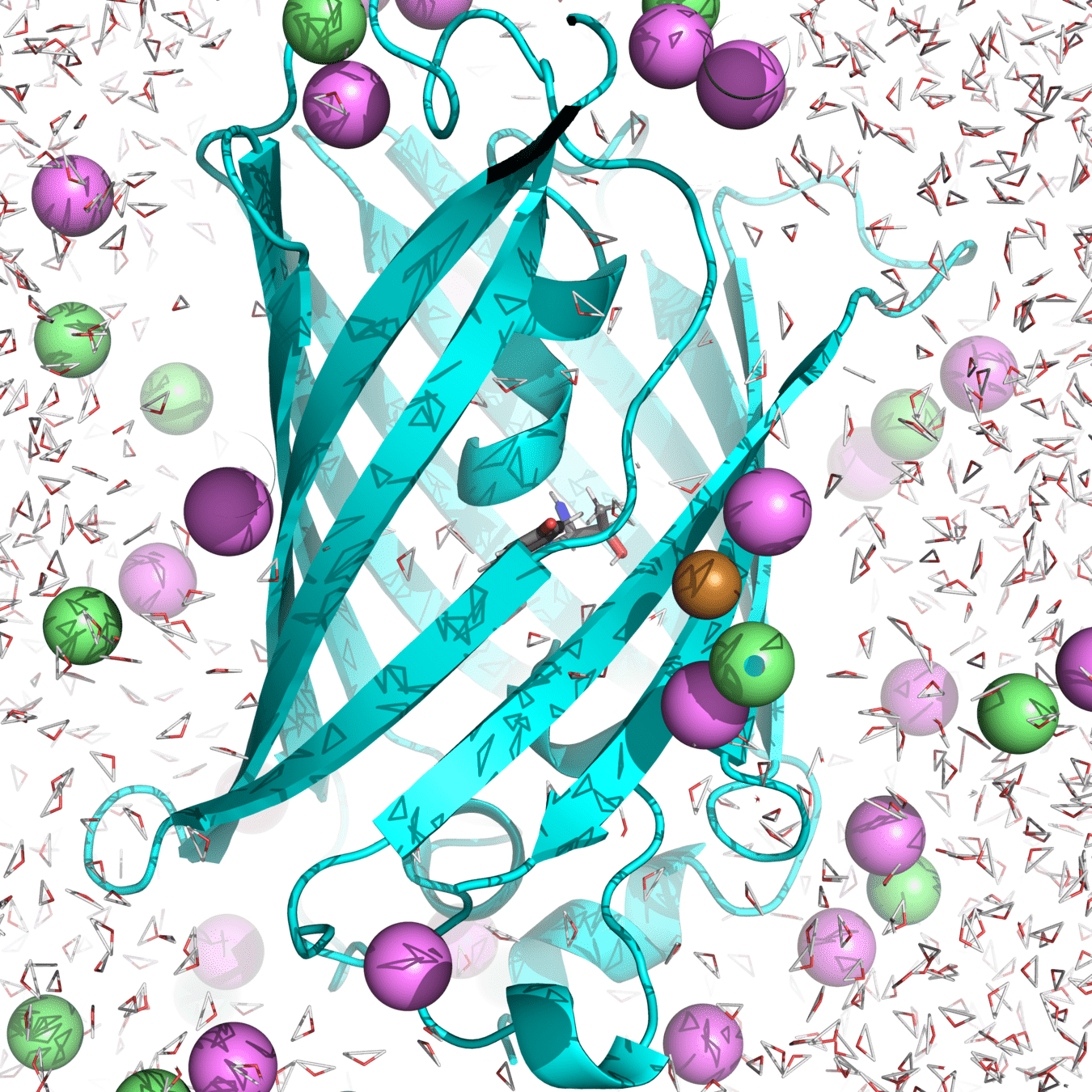
Ensemble example: roGFP2 hydrogen bonding
His148 in GFP stabilizes the anionic chromophore through a hydrogen bond


Let's use MD simulations to compute hydrogen bond length and energy
How would you approach this?

Compute the mean hydrogen bond length of the macrostate's ensemble
Our macrostate: roGFP2 in water, with 150 micromolar NaCl at 300 K and 1 atm
An ensemble is the collection of all possible microstates of a single macrostate
A microstate is a unique configuration defined by the positions and velocities of all particles
Here is the MD trajectory
What is wrong with this?
with a mean of 3.155 Å
The MD simulation is extremely short
Accurate ensemble averages require sampling every possible microstate
Our previous MD simulation was very short
Longer simulations provide better sampling of microstates and their probabilities
More accurate hydrogen bond distance estimate!
Experiments measure the weighted mean of microstates

Remember: Multiple microstates (i.e., configurations) can have the same distance
We measure the ensemble probability of observing a microstate with value
Expected value of ensemble is computed by weighted mean
Note: Our denominator will always be 1 because we are not using actual partition function
2.946 Å
After today, you should better understand
Maintaining thermodynamic equilibrium
Our molecular simulations need to reproduce the desired ensemble
Microcanonical Ensemble (NVE):
Fixed Number of particles (N), Volume (V), and Energy (E)
Most common
Canonical Ensemble (NVT):
Fixed Number of particles (N), Volume (V), and Temperature (T)
Isothermal-Isobaric Ensemble (NPT):
Fixed Number of particles (N), Pressure (P), and Temperature (T)
What does constant temperature mean?

Here is a plot of simulation temperature during a 500 ps MD simulation at 300 K
Is there something wrong with the simulation?

Talk with your neighbors on what could be wrong with the simulation
Remember: Macrostate observables are ensemble averages
True:
Something is wrong
False:
Nothing is wrong
The instantaneous temperature of microstates will fluctuate, but the ensemble average should be constant
There should be no net flow of energy
Kinetic energy determines temperature
300 K
500 K
Note: 3/2 comes from each degree of freedom (x, y, z)
Boltzmann constant
Temperature in Kelvin
Ensemble average kinetic energy
Particle velocities determine kinetic energy

Every particle does not have the same velocity; they generally follow the Maxwell-Boltzmann distribution
- Most Probable Velocity: The velocity at which the peak of the distribution occurs.
- Average Velocity: The mean velocity of all particles.
- Temperature Dependence: Higher temperatures shift the distribution towards higher velocities.
Mass of each particle
Velocity magnitude
Thermostats adjust the velocities of particles to increase or decrease the system's kinetic energy
Thereby controlling the temperature
Berendsen thermostat: Adjusts the velocities of all particles uniformly based on the current temperature and the target temperature
Velocity scaling factor
current velocity
is computed by
scaling the
slowly/carefully
based on the
temperature deviation
This prevents abrupt changes that could destabilize the simulation
Simple velocity scaling does not generate a true canonical (NVT) ensemble; it cannot reproduce realistic temperature fluctuations
Particle collisions are mass dependent
Berendsen thermostats inaccurately models thermal energy transfer via particle collisions
Momenta scaling provides realistic kinetic energy and thus temperature control
This is the principle behind the Nosé-Hoover thermostat
If two particles of different masses collide, will their velocities scale in the same way?
No
1
2
Nosé-Hoover thermostat connect particle momenta to a fictitious heat bath

Momenta adjustment:
This heat bath allows thermal energy to flow in and out of our simulation
"Friction" coupling constant:
is a "mass" coupling parameters that controls thermostat responsiveness
Barostats maintain desired pressure during simulations
Adjusts the volume of the simulation box to achieve and maintain target pressure
Virial corrections to real gas
Corrects for intermolecular forces
Represents thermal energy of ideal gas
Assumes (1) non-interacting particles and (2) elastic collisions
Pressure is directly proportional to density and temperature
Berendsen Barostat: Gentle Pressure Stabilization
Same concept as Berendsen thermostat: Scale box volume based on pressure difference to target
Atomic positions get scaled with box size
Velocities do not get affected


With thermostats and barostats we can keep a consistent macrostate
After today, you should better understand
Relaxation and production MD simulations
Initial configurations are not in true thermodynamic equilibrium
Remember: Starting structures often come from experiments not relevant for our simulation


After minimization, we run a short simulation to let the system adjust to the desired macrostate
We discard the initial relaxation as it is not our desired macrostate

Once our macrostate variable(s) reach steady state, we are now sampling valid microstates

Production simulations sample microstates from our desired macrostate

Remember: Ensemble averages improve with more simulation time by sampling additional microstates
"Replicates" do not exists as it does in experimental biology and chemistry
Multiple shorter simulations or one long one?
Which simulation protocol provides better sampling of microstates?

Assume: Each simulation starts with the same structure, but different initial velocities
Option 1
Three simulations of 500 ns each
Option 2
One simulation of 1,500 ns
Option 1 is correct
Random initial velocities provide better chance of sampling different microstates

Suppose the initial velocities send it in
this direction
Suppose my simulation starts
here
on my potential energy surface (PES)
There is a chance that it never samples this minima
Multiple simulations
with random velocities reduces this chance
After today, you should better understand
RMSD and RMSF as conformational changes and flexibility metrics
Root Mean Square Deviation (RMSD): Monitoring Global Conformational Changes
RMSD measures the overall change in the structure during a simulation, tracking deviations from the starting conformation
The difference between the coordinates represents the displacement of atom iii from its reference position at time ttt
- A low RMSD means the structure is very similar to the reference structure (e.g., stable conformation)
- A high RMSD indicates significant deviation, suggesting large structural changes or flexibility over time
Number of atoms to compare
Position of atom i at time t
Reference position of atom i
Example RMSD plot

Root Mean Square Fluctuation (RMSF): Tracking local flexibility
RMSF identifies regions of flexibility in the protein by calculating the fluctuation of each atom or residue
This measures how much the atom is fluctuating around its mean, not relative to a reference structure
- A high RMSF value for an atom means that it fluctuates a lot, indicating flexibility (often seen in loops or solvent-exposed regions)
- A low RMSF value means the atom remains relatively fixed in place, suggesting rigidity (common in well-ordered regions like helices or beta-sheets)
Total number of time frames
Position of atom i at time t
Average position of atom i
Example RMSF plot


Regions in red have high flexability
LID is an ATP binding domain
NMP is an ADP binding domain
Adenylate kinase (AdK), a phosophotransferase enzyme
After today, you should better understand
Relationship between probability and energy in simulations
What is Potential of Mean Force (PMF)?
PMF represents the effective potential that governs the behavior of a system along a collective variable
- W(x) is the PMF as a function of the collective variable xxx.
- kBk_BkB is the Boltzmann constant.
- TTT is the temperature.
- P(x)P(x)P(x) is the probability of observing a microstate with the collective variable value of xxx.
A collective variable defines the progress of an interaction or molecular reaction
Common collective variable include distances between atoms, bond angles, or dihedral angles.
Interpreting a 1D potential energy surface (PES)

This 1D PES comes from 1500 ns of roGFP2 simulation data
| System | ΔG [kcal/mol] |
|---|---|
| Reduced | -0.559 |
| Oxidized | -1.329 |
| Cu(I) | -0.282 |
His148 in GFP stabilizes the anionic chromophore

Probability and energy are intricately linked


Probability density
Energy
Before the next class, you should
- Turn in A05
- Start A06
Lecture 15:
Ensembles and atomistic insight
Today
Tuesday
Lecture 16:
Structure-based drug design