

Computational Biology
(BIOSC 1540)
Oct 29, 2024
Lecture 16:
Structure-based drug design
Announcements
-
A06 is due Thursday by 11:59 pm
- Reminder: There is a (soft) limit of 100 words for each question
- A07 (final assignment) will be released Friday
- No class on Nov 5 for election day
- The next exam is on Nov 14
- We will have a review session on Nov 12
- Request DRS accommodations if needed
- Project will be released Nov 21 and is due on Dec 10

After today, you should better understand
Drug development pipeline
Drug development is a complex, multi-stage process requiring significant time and resources

1. Discovery and Preclinical Research
Potential drugs are identified and tested in non-human studies
2. Clinical Trials
Testing in human subjects to assess safety and efficacy
3. Regulatory Approval
Evaluation by agencies like the FDA before the drug can be marketed
4. Post-Marketing Surveillance:
Ongoing monitoring after the drug is available to the public
Computation is most helpful with the drug discovery stage
Identifying the right protein target is crucial for developing effective and safe drugs
Proteins regulate nearly all cellular processes and drugs can inhibit or activate proteins to correct disease states
Criteria for Selecting a Protein Target
- Disease Relevance: The protein plays a critical role in the disease mechanism.
- Druggability: The target has a structure that allows it to bind with drug-like molecules.
- Specificity: Targeting the protein minimizes effects on healthy cells, reducing side effects.
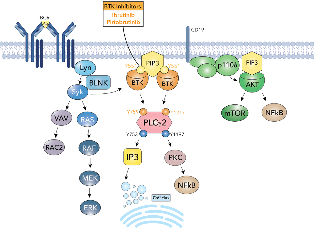
Example: Bruton’s tyrosine kinase (BTK) is a critical signaling enzyme that controls B-cell development, maturation, and activation by mediating B-cell receptor signal transduction
Now we can use ...
BTK gene was implicated in X chromosome-linked agammaglobulinemia (XLA)
Target identification is accelerated with bioinformatics
Genome-wide association studies, high-throughput screening
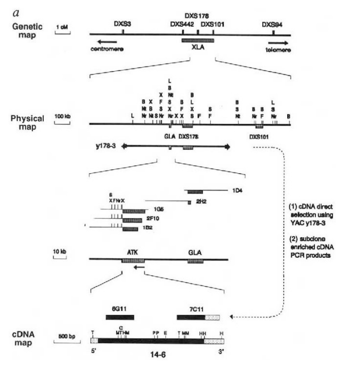
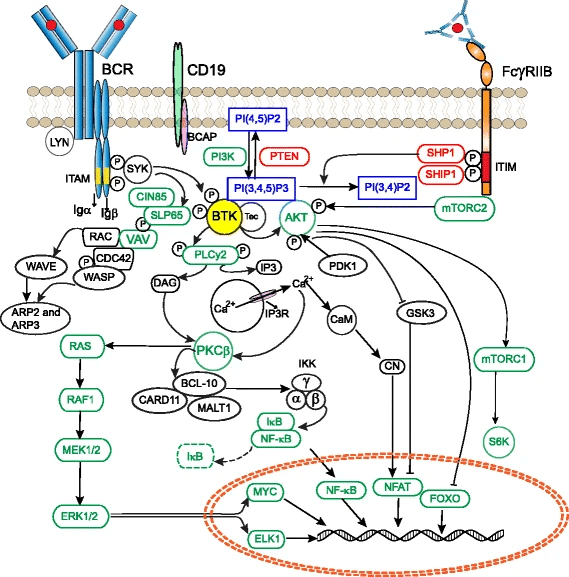
Revealed that BTK as a central hub in B-cell receptor (BCR) signaling
Target identification is accelerated with bioinformatics
Now we can use ...
Proteomics, transcriptomics
With a protein target in hand, we can now identify potential drug candidates
After today, you should better understand
Role of structure-based drug design
Chemical space contains an astronomical number of possible compounds to explore
Effective drugs must bind to the target protein with sufficient affinity and specificity
Estimated to be between 1060 to 10200 possible small organic molecules
We need methods to navigate chemical space and identify promising leads accurately and efficiently
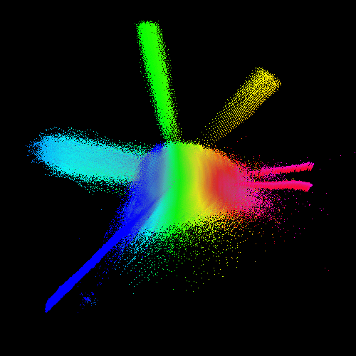
High-throughput screening (HTS) allows testing of thousands of compounds against the target protein
- Library Preparation: Collection of diverse compounds
- Assay Development: Design of biological assays to measure compound activity against the target
- Screening: Compounds are tested in miniaturized assays
- Data Analysis: Identification of "hits" that show desired activity
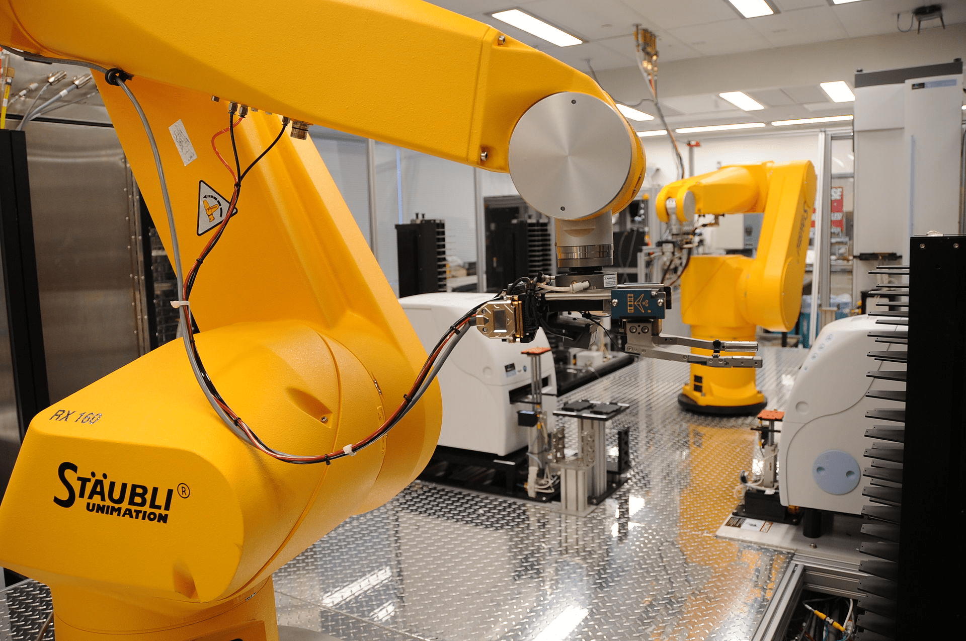
Virtual screening evaluates vast libraries to identify potential leads efficiently
Experimental assays are still expensive, and limited to commercially available compounds
Instead, we can use computational methods to predict which compounds we should experimental validate
Can screen millions to billions of compounds in silico, thereby dramatically expanding our search space

After today, you should better understand
Thermodynamics of binding
Selective binding to a protein is governed by thermodynamics (and kinetics)
Binding occurs when a compound/ligand interacts specifically with a protein
Protein
Ligand
Binding
Protein-
ligand
We can model this as a reversible protein-ligand binding
Binding affinity is determined by the Gibbs free energy change
The change in free energy when a ligand binds to a protein
Determines binding process spontaneity
Gibbs free energy combines enthalpy and entropy
Entropy
Enthalpy
Accounts for energetic interactions
How much conformational flexibility changes
Note: Simulations capture free energy directly instead of treating enthalpy and entropy separately
After today, you should better understand
Enthalpic contributions to binding
Enthalpy accounts for noncovalent interactions
Noncovalent interactions: Electrostatics, hydrogen bonds, dipoles, π-π stacking, etc.

Ensemble differences in noncovalent interactions provide binding enthalpy
Ensemble average
Chemical interactions are determined by fluctuating electron densities
Our noncovalent interactions conceptual framework:
3. Regions of increased electron density are associated with higher partial negative charges
4. Electrons are mobile and can be perturbed by external interactions
1. Coulomb's law describes the interactions between charges
Molecular interactions are governed by their electron densities (Hohenberg-Kohn theorem)
This is rather difficult, so we often use conceptual frameworks to explain trends (e.g., hybridization and resonance)
2. Molecular geometry uniquely specifies an electron density
Electrostatic forces govern interactions between charged and polar regions
Charged molecules have a net imbalance between
- Positive charges in their nuclei
- Negative charges from their electrons
This leads to net electrostatic attractions or repulsions between different atoms or molecules
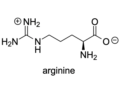
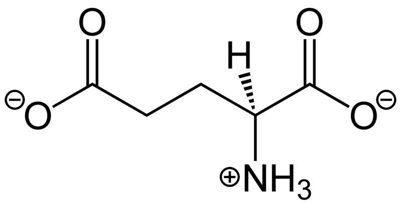
Arginine
Glycine
~5 to 20 kcal/mol per interaction
Long-Range Interaction: Can attract ligands to the binding site from a distance
Anchor Points: Often serves as key anchoring interactions in the binding site
Role in binding
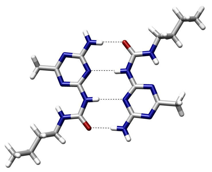
Hydrogen bonds are a type of electrostatic interactions
Attraction between a (donor) hydrogen atom covalently bonded to an electronegative atom and another (acceptor) electronegative atom with a lone pair
- Common donors: O-H, N-H groups
- Common acceptors: O and N atoms with lone pairs
~2 to 7 kcal/mol per hydrogen bond
Strongest when the hydrogen, donor, and acceptor atoms are colinear
Specificity: Precise orientation of the ligand
Stabilization: Moderately strong interactions
Role in binding
Dynamic: Allows for adaptability of ligands
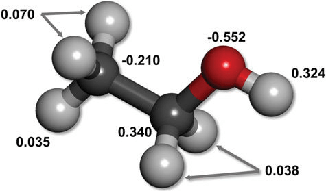
Uneven electron distribution creates partial charges and dipoles
Electronegativity differences lead to unequal distribution of electron density
Unequal distribution results in regions or partial positive or partial negative charges
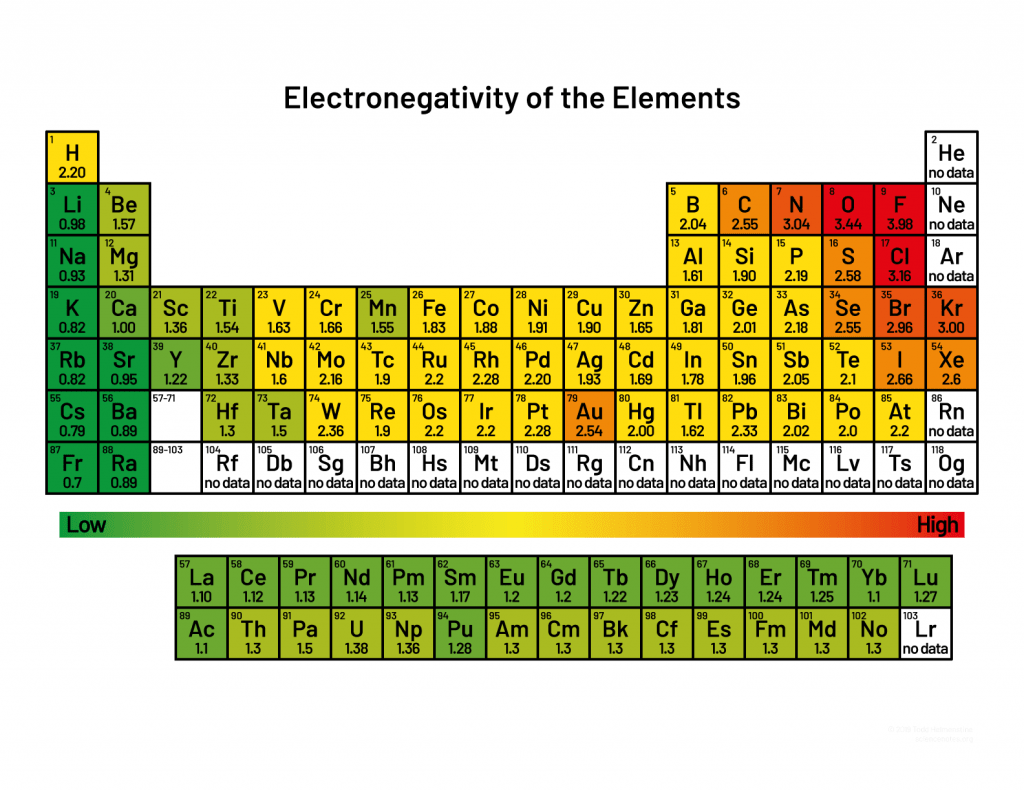
Consistent electron density spatial variation results in permanent dipoles
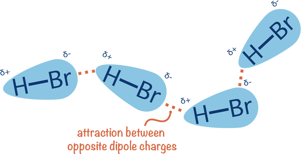
~0.01 to 1 kcal/mol per interaction
Directional binding: Highly directional, ensuring that the ligand aligns correctly
Flexibility: Can accommodate slight conformational changes
Role in binding
Van der Waals forces are weak, non-directional interactions
Dispersion: Electrons in molecules are constantly moving, leading to temporary uneven distributions that induce dipoles in neighboring molecules
~0.4 to 4 kcal/mol per interaction
Complementary fit: Maximizes surface contact
Flexibility: Allows small conformational changes
Role in binding
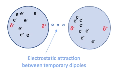
Induction: The electric field of a polar molecule distorts the electron cloud of a nonpolar molecule, creating a temporary dipole
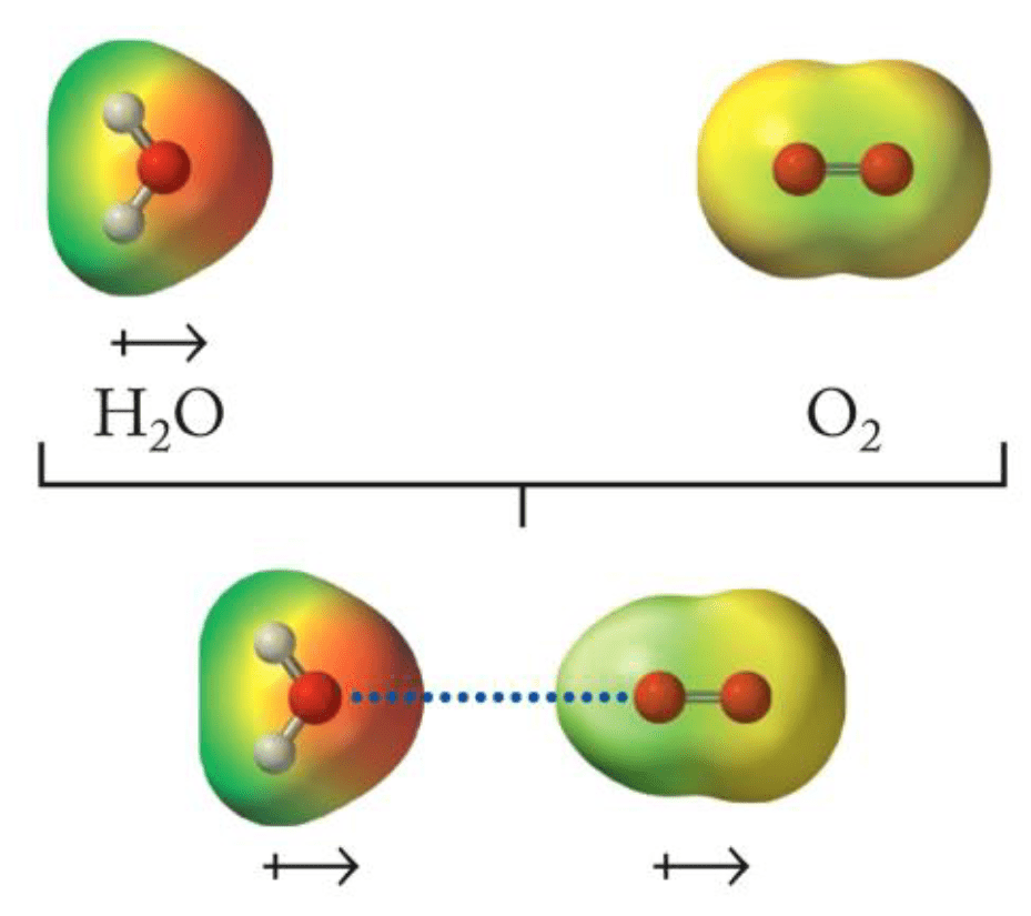
π-π interactions involve stacking of aromatic rings
Noncovalent interactions between aromatic rings due to overlap of π-electron clouds
~1 to 15 kcal/mol per interaction

Edge-to-face


Displaced
Face-to-face
Orientation: Proper positioning of aromatics
Selectivity: Recognition of ligands
Role in binding
Summing all of these contributions during a simulation provides our ensemble average
After today, you should better understand
Entropic contributions to binding
Entropy accounts for microstate diversity of a single system state
One of Alex's esoteric points: "Entropy is disorder," is a massive oversimplification that breaks down in actual practice
Entropy is formally defined as
is the total number of microstates available to the system without changing the system state
Entropy is "energy dispersion"
Higher entropy implies greater microstate diversity
"System state" can be arbitrarily defined and compared as
- Unbound ligand vs. bound ligand
- Unfolded protein vs. folded protein
- Liquid water at 300 K vs. 500 K
Grid-based protein-ligand binding
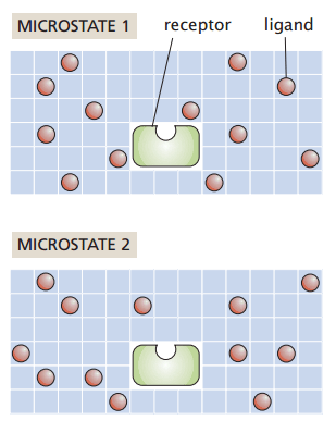
Suppose I have a system with
- Protein receptor
- Ligands positioned on a grid
My macrostate (number of particles, temperature, and pressure) remain constant
How many ways can I rearrange the ligands without binding to the receptor?
Number of ligands
Number of sites
Number of ways to choose L grid sites out of N is the binomial coefficient
Grid-based protein-ligand binding
What if one ligand binds to the receptor?
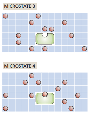
How does entropy change?
Increase
No change
Decrease
It depends on our ligand concentration!
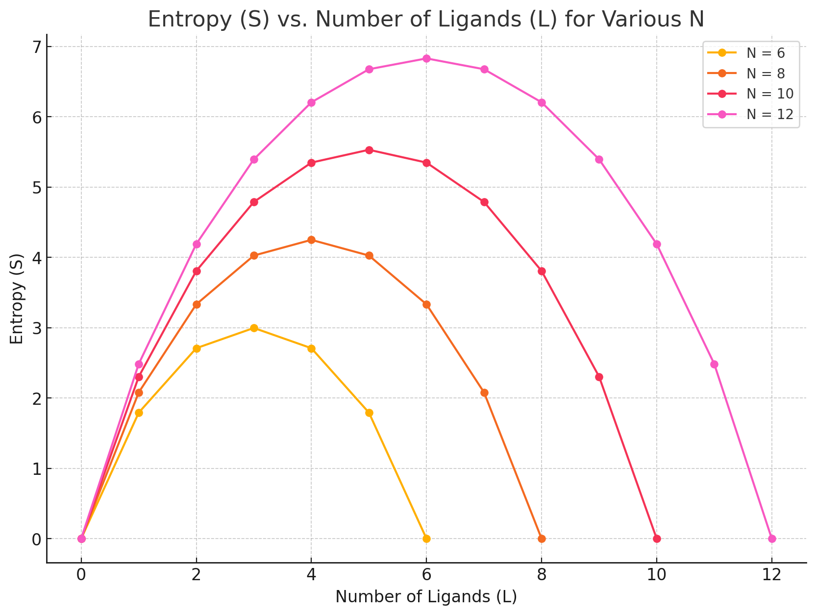
How to interpret this: Pick a number of ligands and move to the right (L - 1), does entropy go up or down?
For protein-ligand binding, we need to account for how the number of accessible microstates/configurations for protein and ligand

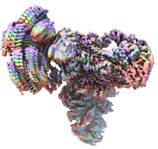
After today, you should better understand
Alchemical free energy simulations
We can now run molecular simulations of different states
To compute the free energy of a "system state", we have to compute the state's partition function, Z
We can run simulations and directly compute the ensemble average free energy
This is theoretically valid but not practical. Why?
Exact partition functions include all microstates
To compute the partition function of protein; for example, we need to know the energy for
- All possible conformations (folded, partially folded, unfolded)
- All possible atomic positions (backbone and sidechains)
- All possible velocities of the atoms
- All possible rotational states
- All possible vibrational states
This is impossible
Fortunately, the low-energy conformations contribute the most to the partition function
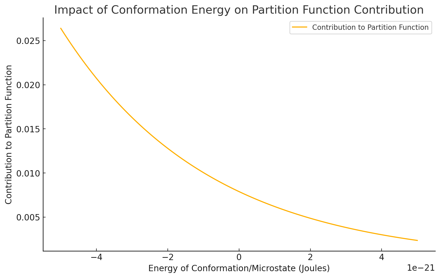
Molecular simulations can sample some low-energy conformations; however, minor errors will drastically impact absolute free energy calculation
What if we slowly disappear the ligand?
We could use an alchemical parameter, , to scale noncovalent interactions between protein and ligand
This allows us to sum relative free energies to estimate amount of energy to bind/unbind the ligand
How does this help us?
Relative free energies are expressed as a partition function ratio
The free energy change from state A to B can be computed as
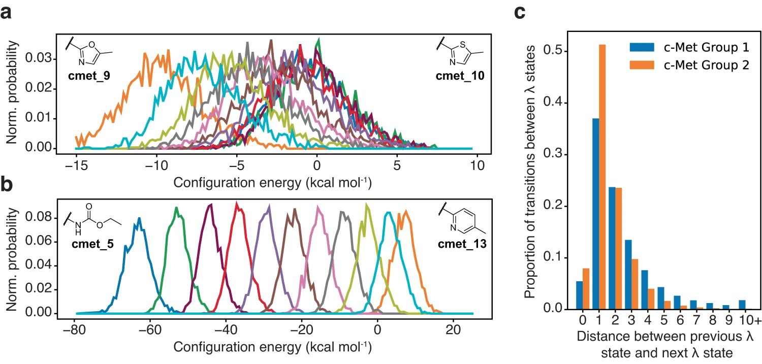
Advantage: Partition function ratios are dominated by overlapping microstates common between states A and B
Maintaining phase space overlap ensures more reliable and converged free energy estimates
(This is conceptually similar to having a small integration step size.)
Thermodynamic integration provides a way to compute free energy differences
We can to integrate over these small free energy changes
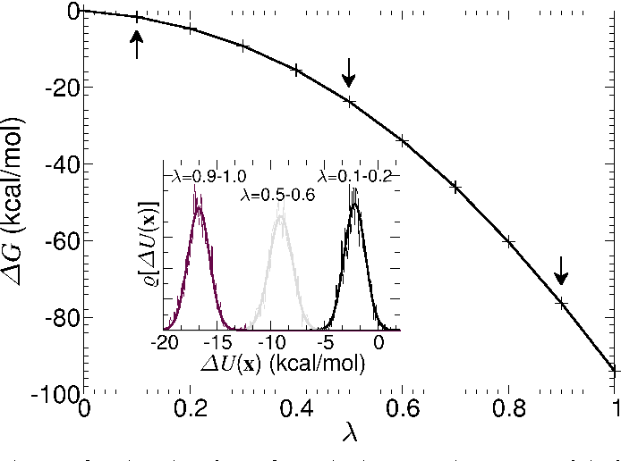
We can use this to reliably calculate the free energy difference between bound and unbound states
Alchemical simulations are actually very expensive
We use "docking" to more efficiently screen molecules before (if ever) doing alchemical simulations
Before the next class, you should
Lecture 16:
Structure-based drug design
Today
Thursday
Lecture 17:
Docking and virtual screening
The partition function is the sum of all energy-weighted microstates
Let's go back to our grid model with two system states: (A) unbound and (B) bound
Note: To make our lives easier, we assume each microstate has the same energy
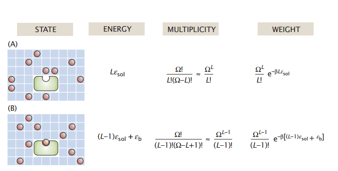
Energy
State
Multiplicity
Weight
The Stirling approximation
Energy
of each microstate. (In our model, this is based on number of solvated and bound ligands)
The of this system state in our macrostate ensemble
weight
Total partition function
Multiplicity
, or the the number microstates
So, what's the issue with computing this for each state?