Introduction to epigenetics and ChIP-Seq
Aleksandra Galitsyna
“Analysis of omics data” course
Skoltech
24 February 2022

Introduction: sequencing
"Computational analysis of
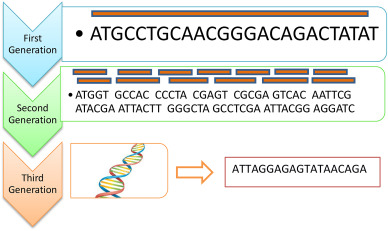
Sanger
Illumina, Roche 454, SOLiD
Nanopore
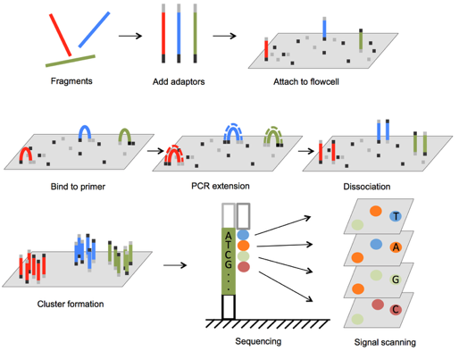
Illumina sequencing
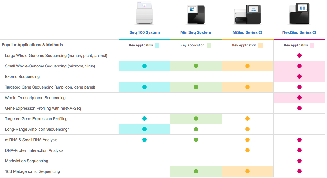
Illumina sequencers

NGS techniques diversity
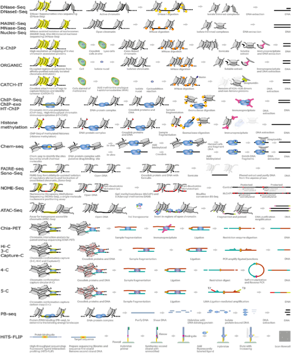
Wasserman & Sandelin. Applied bioinformatics for the identification of regulatory elements. Nat. Rev. Genet. 2004
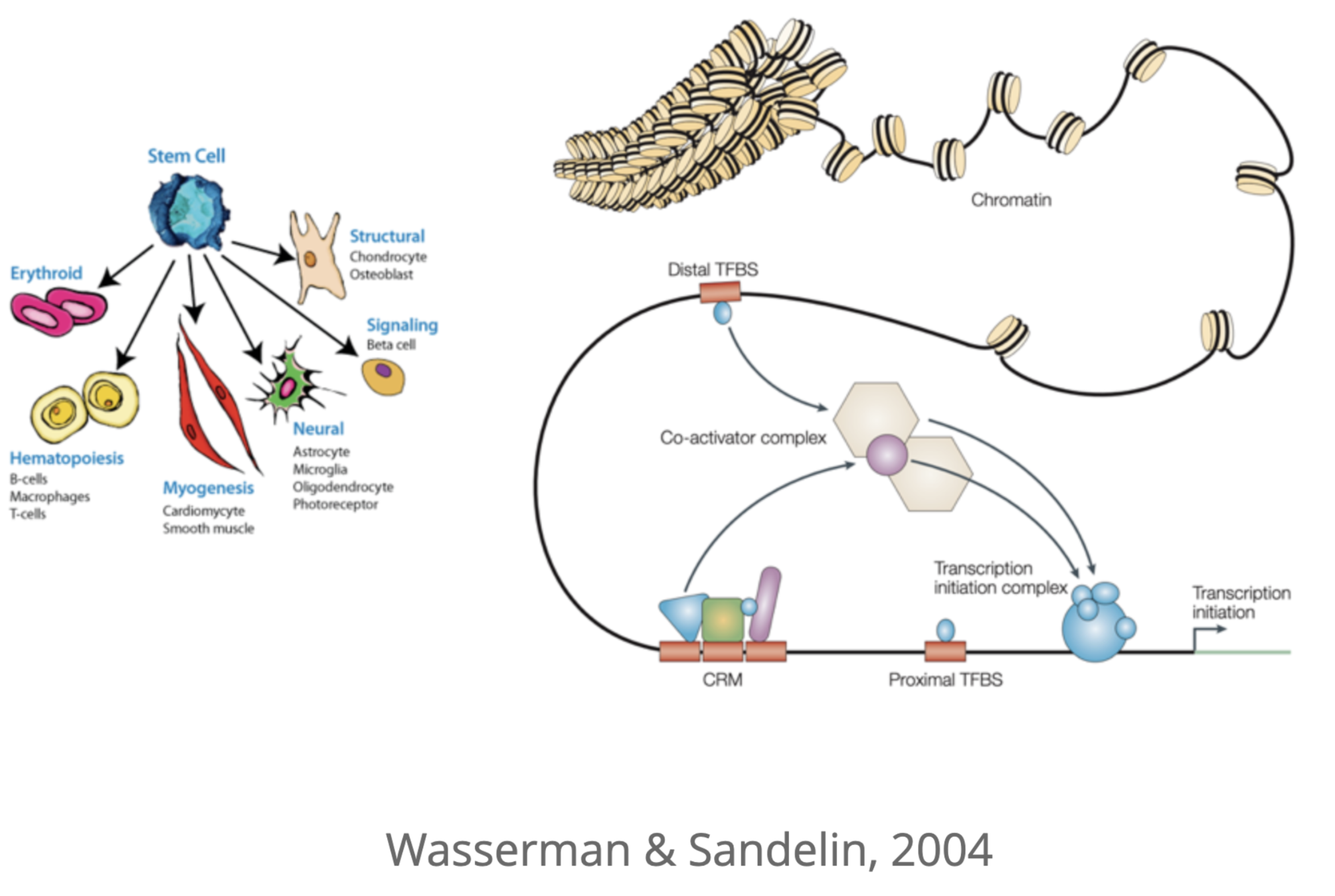
Activation of promoters and enhancers
Key determinant of expression is activation of promoters and enhancers
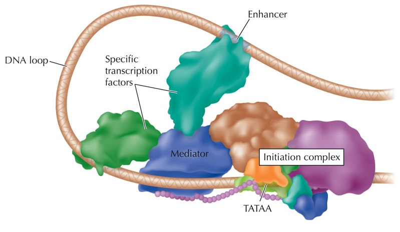
Promoter

How to activate enhancer and promoter?
Regulatory networks of enhancers
One gene can regulate multiple enhancers,
while multiple enhancers can influence a gene:
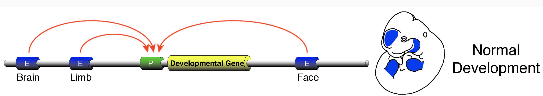
Wasserman & Sandelin. Applied bioinformatics for the identification of regulatory elements. Nat. Rev. Genet. 2004
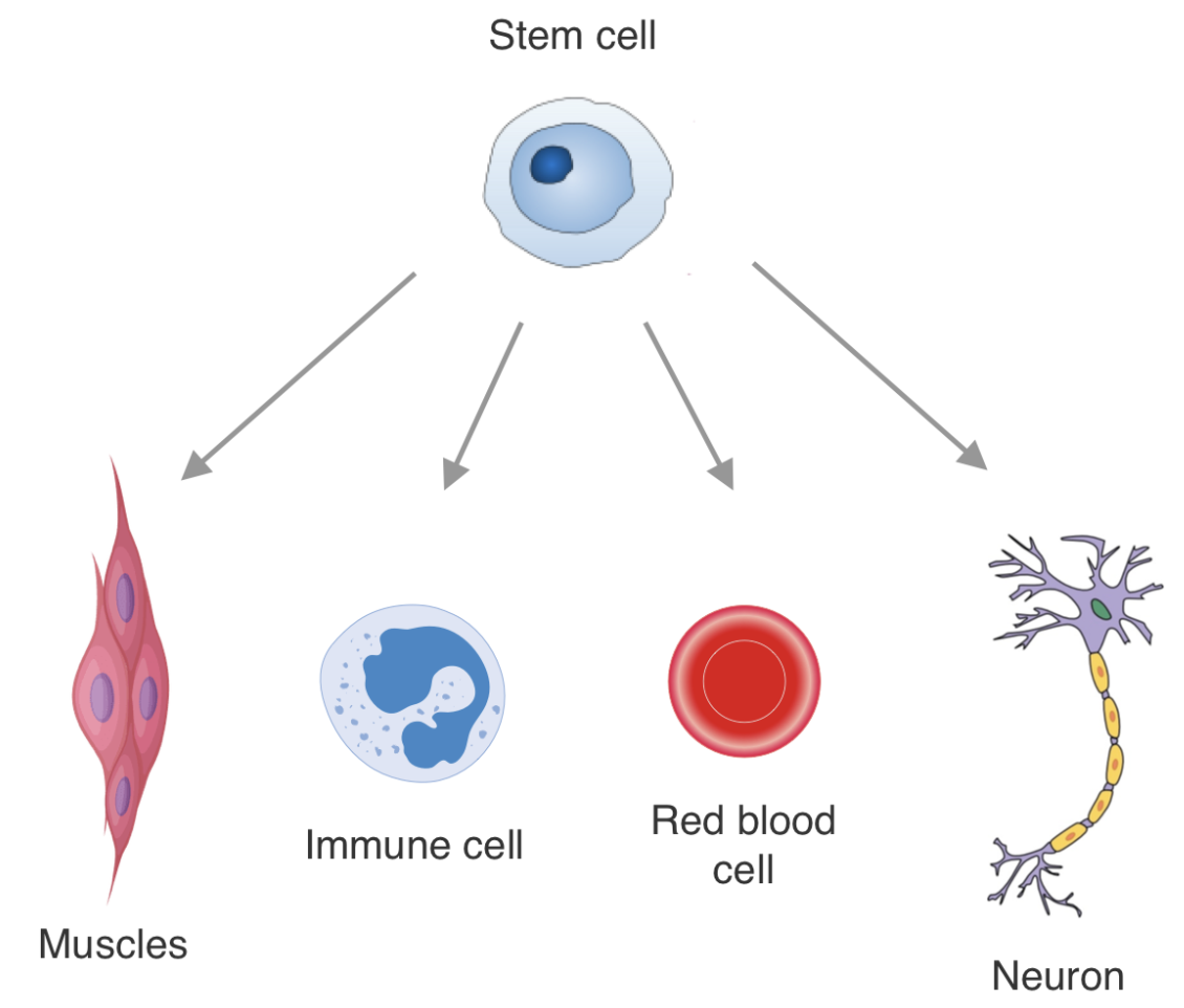
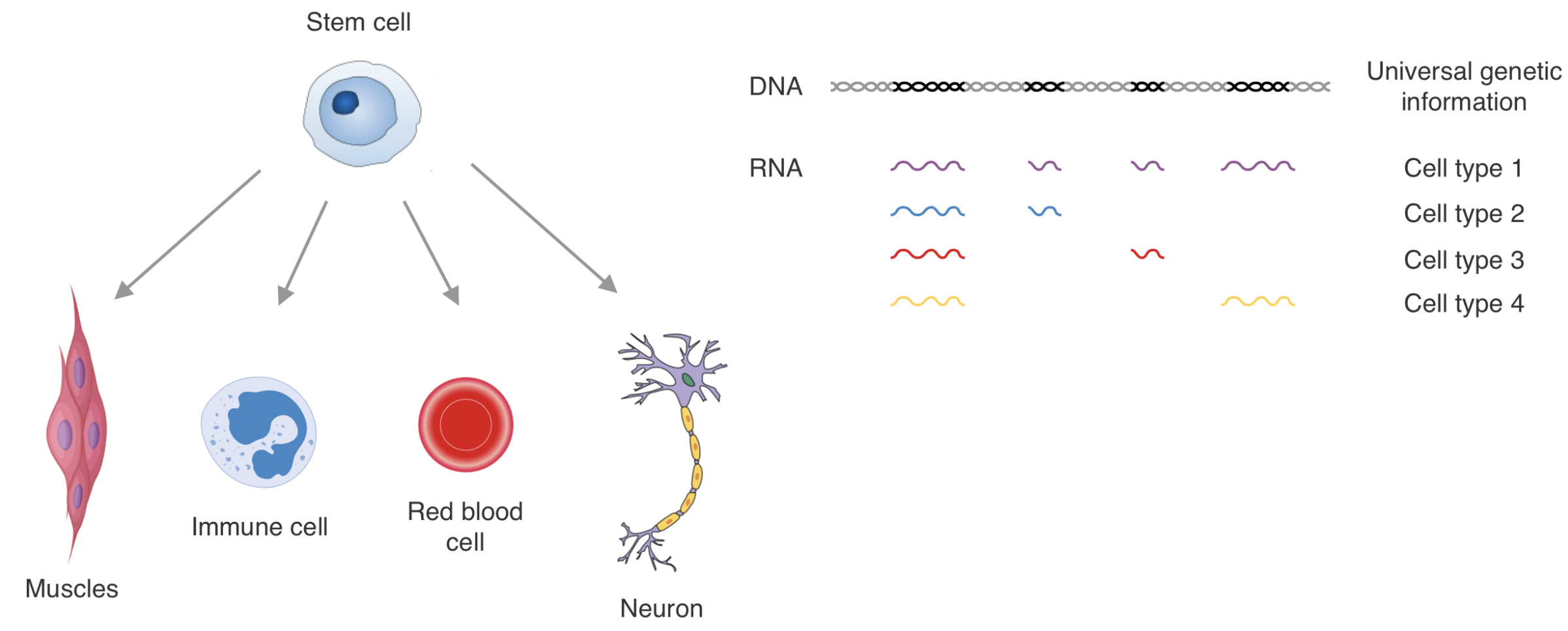
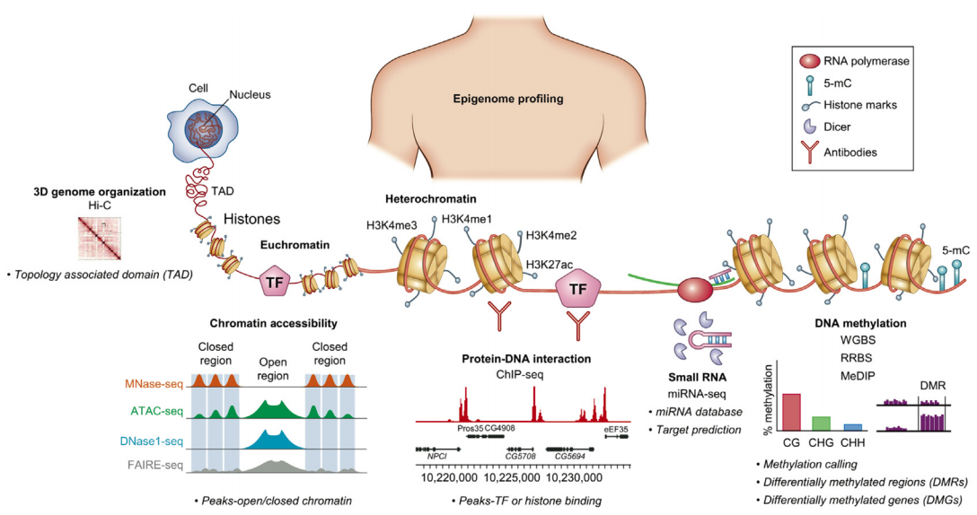
Epigenetic encoding of expression patterns:
Sequencing for epigenetics
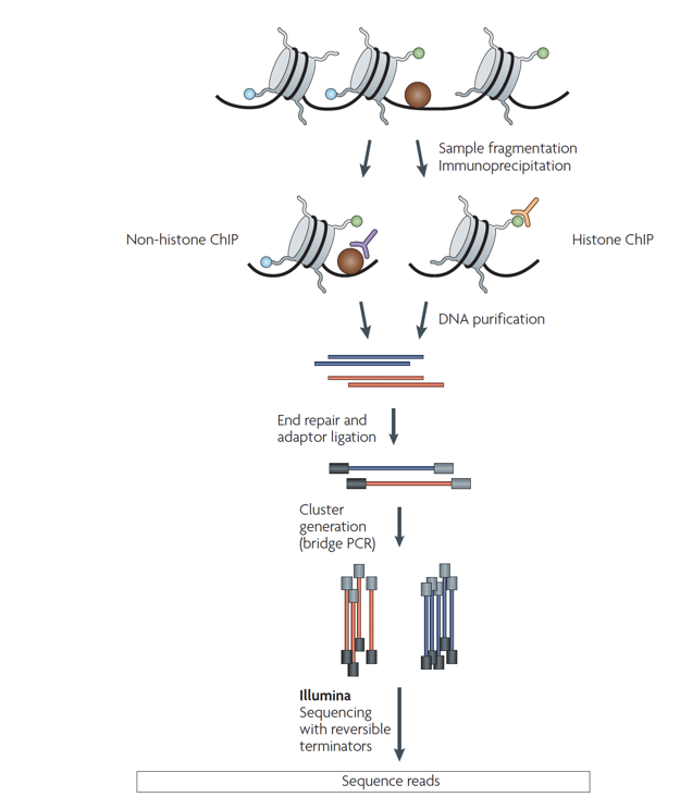
ChIP-Seq: experimental protocol
- Aim: find all regions in the genome bound by a specic transcription factor (or bearing a specic histone modication)
- Answer: ChIP-Seq, Chromatin immunoprecipitation with sequencing
Park 2009
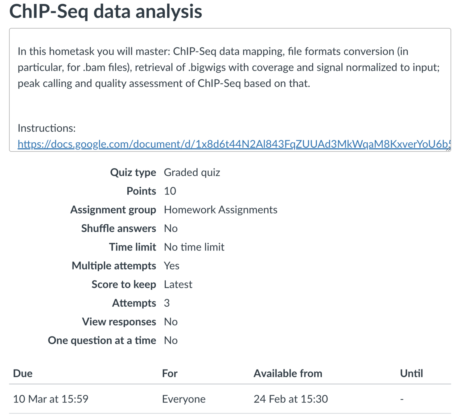
Practice
Before we start the practice...
- Hometask made available on canvas:
- Find and follow the instructions for the seminar here
Before we start the practice...
- We will work in browser and with terminal. We also need to copy files from the remote server, so install appropriate software, if needed (your favourite terminal distributive,
Putty: https://www.putty.org/ or WinSCP: https://winscp.net/eng/download.php) - File formats are specified after the dot (e.g. .bam).
- Code is running in grey boxes with monospace font, try not to copy it blindly, because:
some file names are surrounded by brackets "${}". This indicates that it should be replaced by the name of your file. You may use the filenames that you like, but I highly recommend to stick to using the name of your factor and input instead.
echo "Bioinformatics has never been easier! Copy&paste wisely, or rm -rf ~/ will strike you one day."
Before we start the practice...
Review of some useful bash commands:
- List files in the current directory:
- Check the current position in the directory tree:
- Open text file for reading:
- Run command help, one of the options:
(some of them work for ones
but not the others)
- Copy file:
- Enter directory:
- Exit the directory:
- Create directory:
- File decompression:
lspwdless file.txtsome_command -hsome_command --helpman commandcp target_file destination_foldercd directory_name/cd ../ls -htsmkdirgzip -d file.gzunzip file.zipExpected result of the seminar
- Quizz on canvas (10 points in total)
- Extended deadline until 24th of March.
- Each task of the quizz is screenshot + essay answer.
- Mistakes on biology and theory are penalized.
- Feel free to ask the questions in the chat!
ChIP-Seq theory
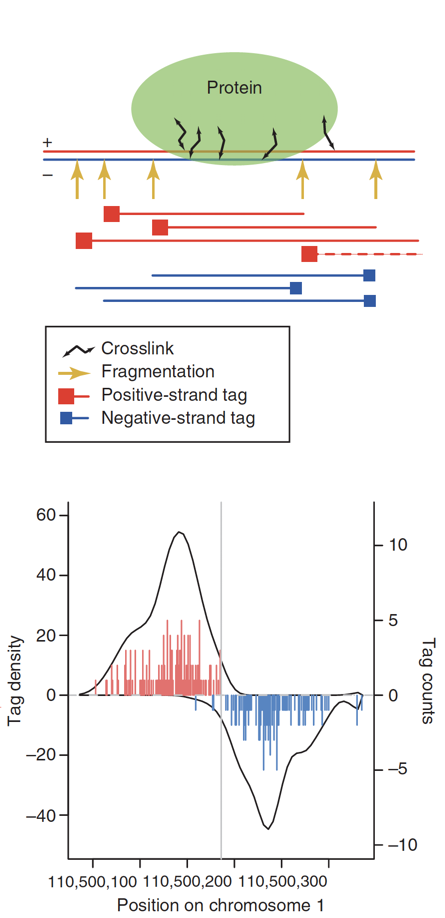
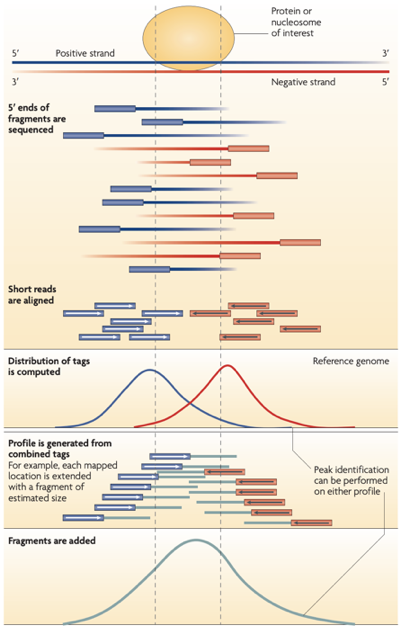
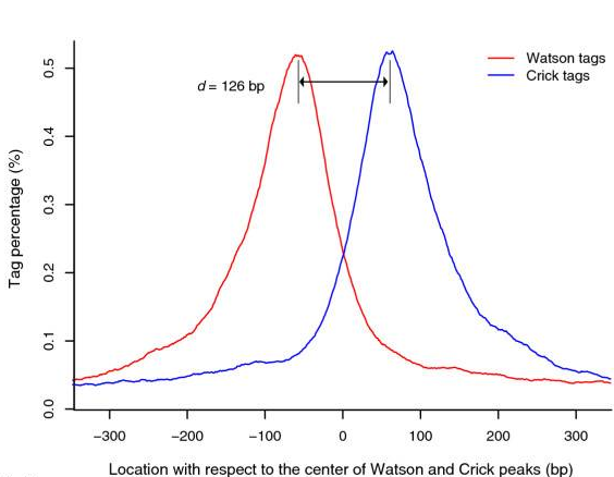
ChIP-Seq: density of DNA fragments
- We expect to find different results for plus (Watson) and minus (Crick) strands of DNA:
Park 2009
ChIP-Seq: Cross-Correlation
- We expect to find different results for plus (Watson) and minus (Crick) strands of DNA:
Park 2009
ChIP-Seq: Cross-Correlation
-
The cross-correlation typically peaks at the shift corresponding to the fragment length and the shift corresponding to the read length.
Bailey 2013

ChIP-Seq: Cross-Correlation measure
-
NSC (normalized strand cross-correlation coefficient):
The ratio between the cross-correlation at the fragment length and the background crosscorrelation. -
RSC (relative strand cross-correlation coefficient):
The ratio between cross-correlation at the fragment length and the crosscorrelation at the read length. -
Very successful ChIP experiments generally have NSC>1.05 and RSC>0.8
Bailey 2013
Input control
- Input experiment is ChIP-Seq control with the same experimental steps but without immunoprecipitation.
- Input is used for normalization of ChIP-Seq.
-
Input experiment accounts for unwanted factors contributing to sequencing & processing output:
- DNA-shearing is not uniform across genome -> more reads in open chromatin regions,
- Amplification bias (GC content),
- Repetitive regions,
- DNA accessibility
Park 2009
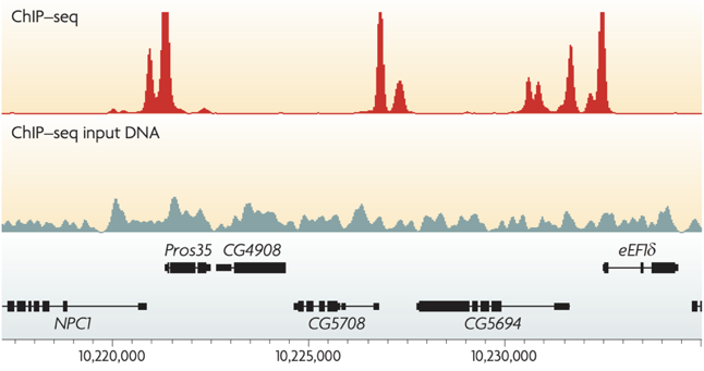
Normalization by input control
Park 2009
elevated
(absolute values)
enriched
(relative to input)
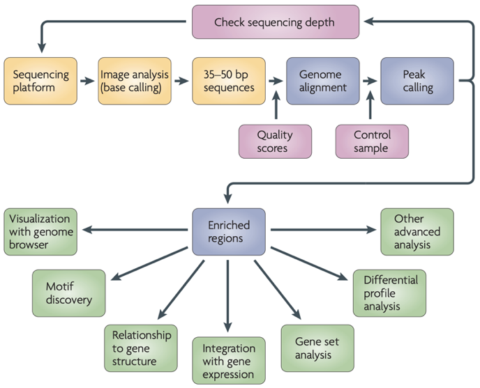
ChIP-Seq data processing
Park 2009
ChIP-Seq data processing: implementation
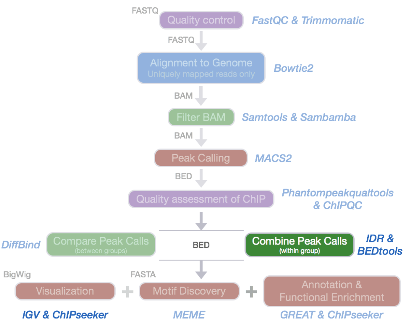
ENCODE Standards:
https://www.encodeproject.org/chip-seq/transcription_factor/
ChIP-Seq peak calling
MACS2 is the most common software:

ChIP-Seq peak calling result
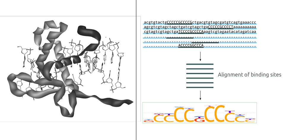
Binding of protein is typically specific to DNA sequence:
ChIP-Seq: peak calling
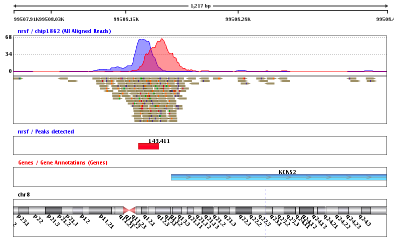
Example output of the procedure:
What is the next step?
Binding events and DNA motifs
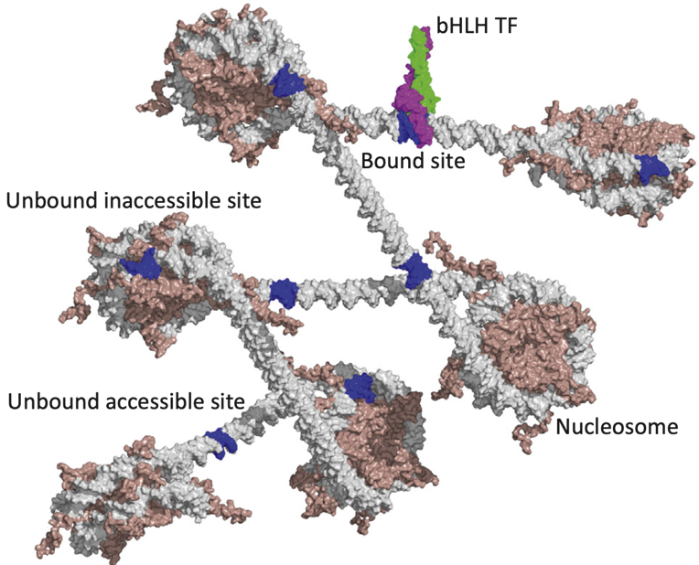
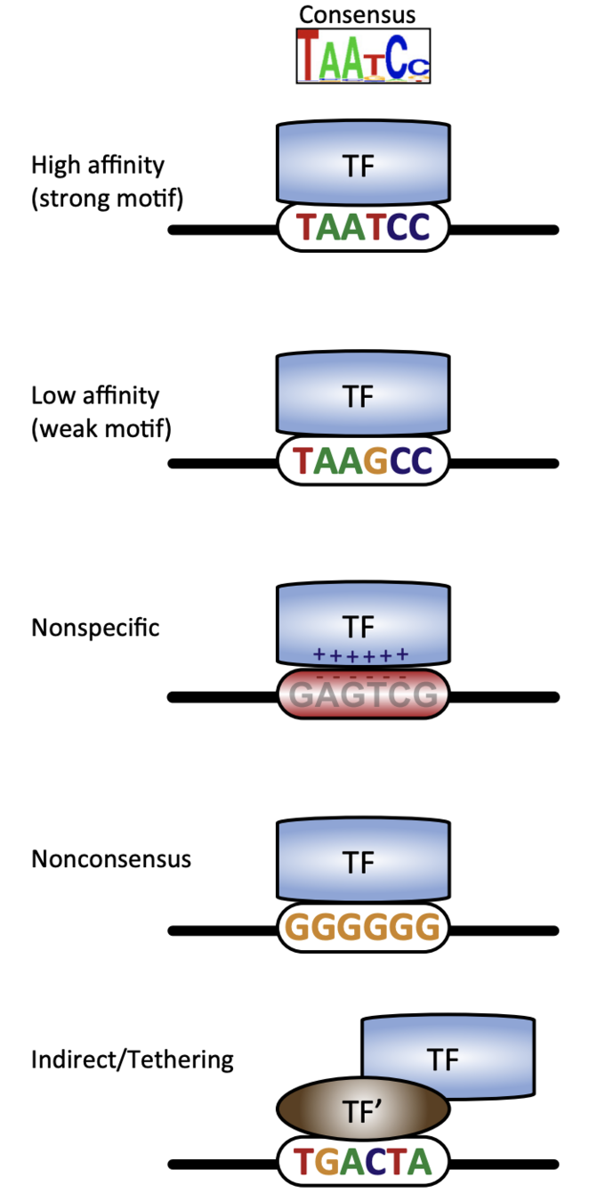
Specific and non-specific binding:
Slattery et al. 2014
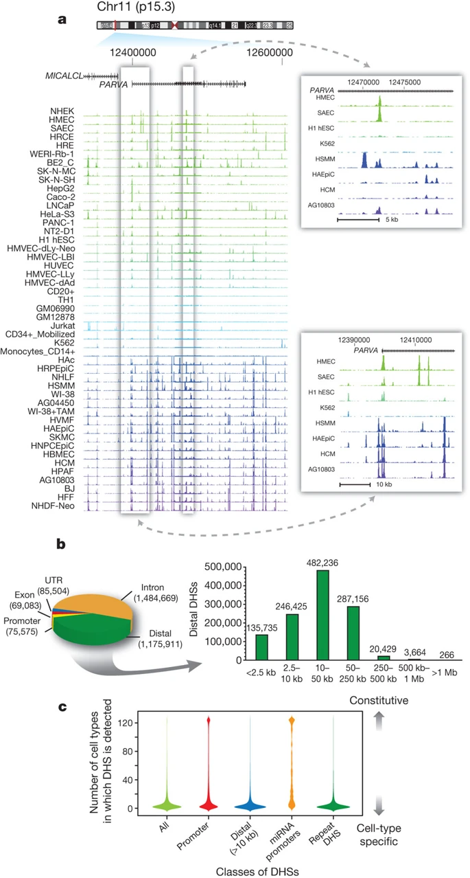
Genomics tracks association
DNase-Seq coverage for ∼350-kb region:
Thurman et al. Nature 2012
Different cell types
Clustering of samples
Cusanovich et al. Cell 2018
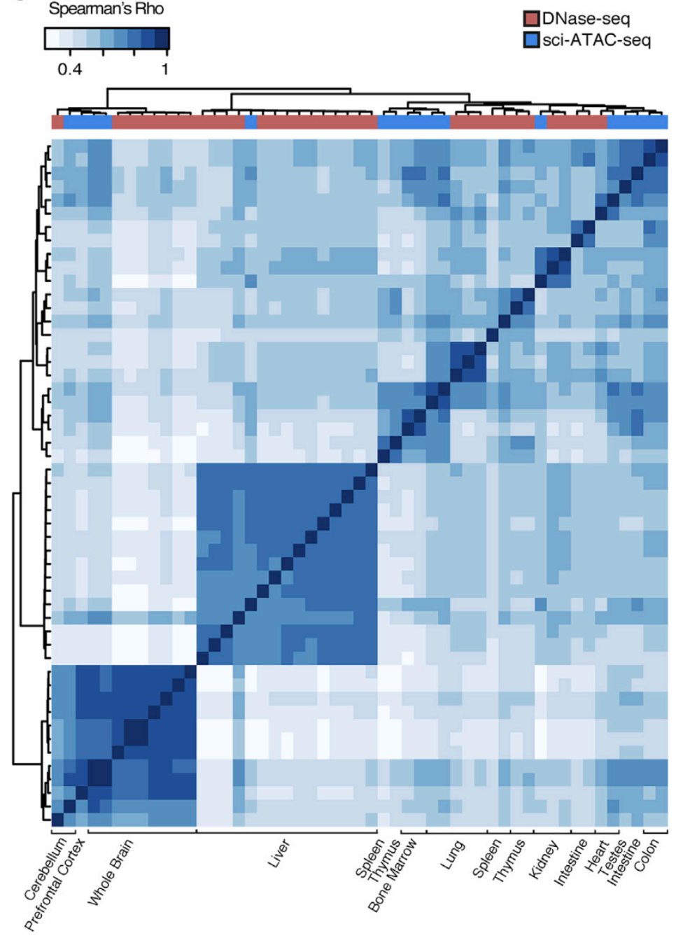
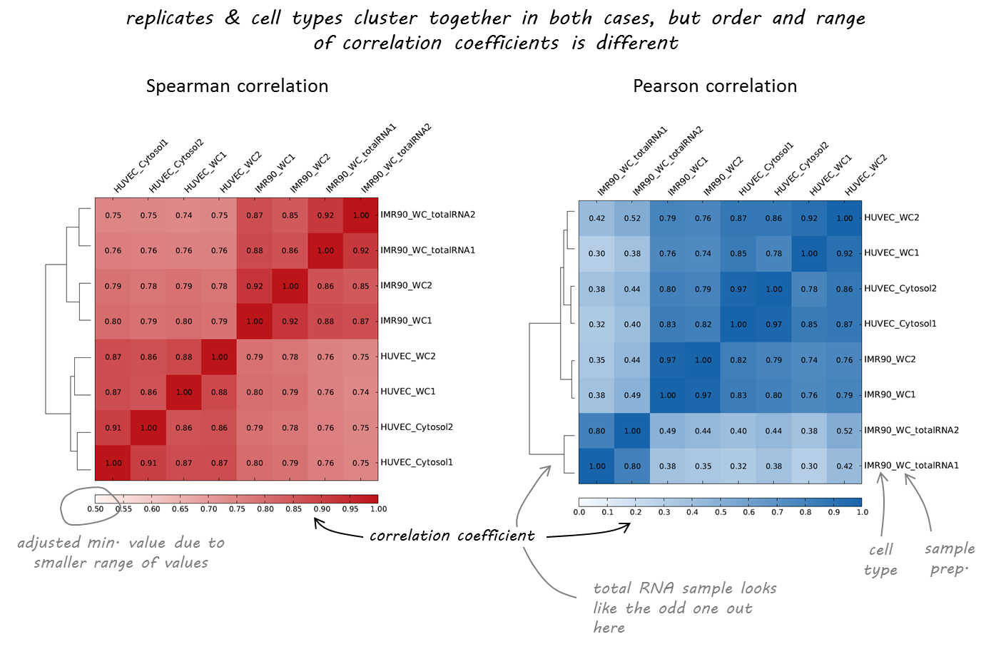
Let's check the similarity of pooled tissue samples with DNase-seq from known tissues. For that, let's plot bi-clustered heatmap of Spearman correlation coefficients:
Result of clustering,
the tree reflecting the similarity between samples
Clustering of samples
Cusanovich et al. Cell 2018
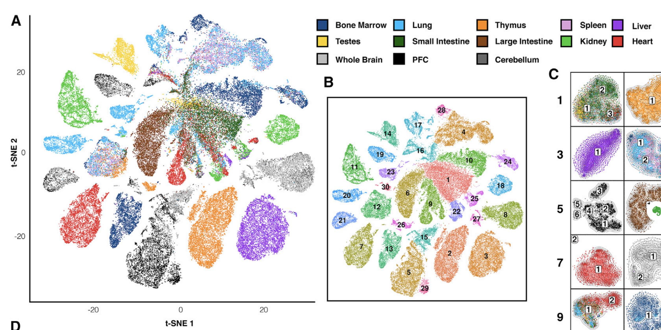
Finally, let's do dimensionality reduction, where each dot is a single sample.
Here is an example with t-SNE, although PCA (Principal Component Analysis) and MDS (Multidimensional scaling) are other popular techniques:
Practical Part: Samples Comparison
We will use deeptools commands multiBigwigSummary and plotCorrelation to compare the ChIP-Seq experiments. We will construct bi-clustered heatmaps of correlations:
Text
Stackup Plots (enrichment profiles):

Additional slides
FYI
Get in touch with your data: step 1
1. Login to the server via terminal:
or use Putty on Windows.
(example instructions https://www.ssh.com/ssh/putty/windows/#sec-Configuration-options-and-saved-profiles)
2. Create the folder with your project:
3. Activate prepared environment:
(if you have problems with it, please, contact the TA)
4. Check your environment:
ssh username@servernamemkdir EpiPract1
cd EpiPract1export PATH="/home/a.galitsyna/conda/bin:$PATH"
conda activate chipseqls # Should list all the filesin the directory
pwd # Should result in your currentl location
conda list # Should list all the programs installed, if conda imported successfully.Get in touch with your data: step 2
- Find your datasets (here or in the table on the right):
- Copy to the local folder:
- Check the content and file sizes:
less /home/a.galitsyna/datamkdir ~/lesson6/
cp /home/a.galitsyna/data/reads/${your_files.fastq.gz} ~/lesson6/cd ~/lesson6
ls -hts Get in touch with your data: step 3
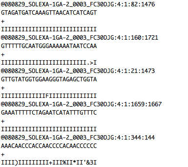
- Open FASTQ files, check the format
(see also: http://emea.support.illumina.com/bulletins/2016/04/fastq-files-explained.html)
- Check FASTQ files, what is the number of rows vs the number of entries?
- Run fastqc (a tool for FASTQ quality control, or QC)
gzip -d <file.fastq.gz> # This will result in <file.fastq> unzipped file
less <file.fastq>
wc -l <file.fastq>fastqc <file.fastq>NGS data typical workflow example
Let's review the NGS data processing workflow:
- Quality control: fastqc on initial FASTQ
- Index build: bowtie2-build on initial chromosomes files
- Read mapping: FASTQ → SAM/BAM
- Filtering of mapped reads: samtools on SAM from p.3
- Conversion to BED: bedtools on SAM from p.4
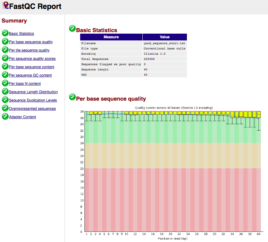
FASTQC report example
- Takes FASTQ as input:
- Output format: html and plain text
fastqc <input.fastq>ls
# input.fastq input_fastqc/
cd input_fastqc/
ls
# fastqc_data.txt fastqc_report.html Icons Images summary.txtDon't run this code, it's FYI
FASTQC report example
- Example html output:
(see https://www.bioinformatics.babraham.ac.uk/projects/fastqc/ for more examples)
Genome index build example
(Manual: http://bowtie-bio.sourceforge.net/bowtie2/manual.shtml)
- Required for fast search of query sequence during mapping
- Takes fasta with reference as input (comma-separated list) and prefix name.
- Example run and resulting database:
bowtie2-build -h

bowtie2-build chr1.fa,chr2.fa,chr3.fa,chr4.fa hg38

# Check the results:

ls -hs

# 938M hg38.1.bt2  701M hg38.2.bt2   12K hg38.3.bt2  701M hg38.4.bt2  3.0G hg38.fa  938M hg38.rev.1.bt2  701M hg38.rev.2.bt2

bowtie2-inspect -n hg38
Don't run this code, it's FYI
Read mapping example
- Takes query FASTQ and indexed database as input.
- Output is in SAM or BAM format
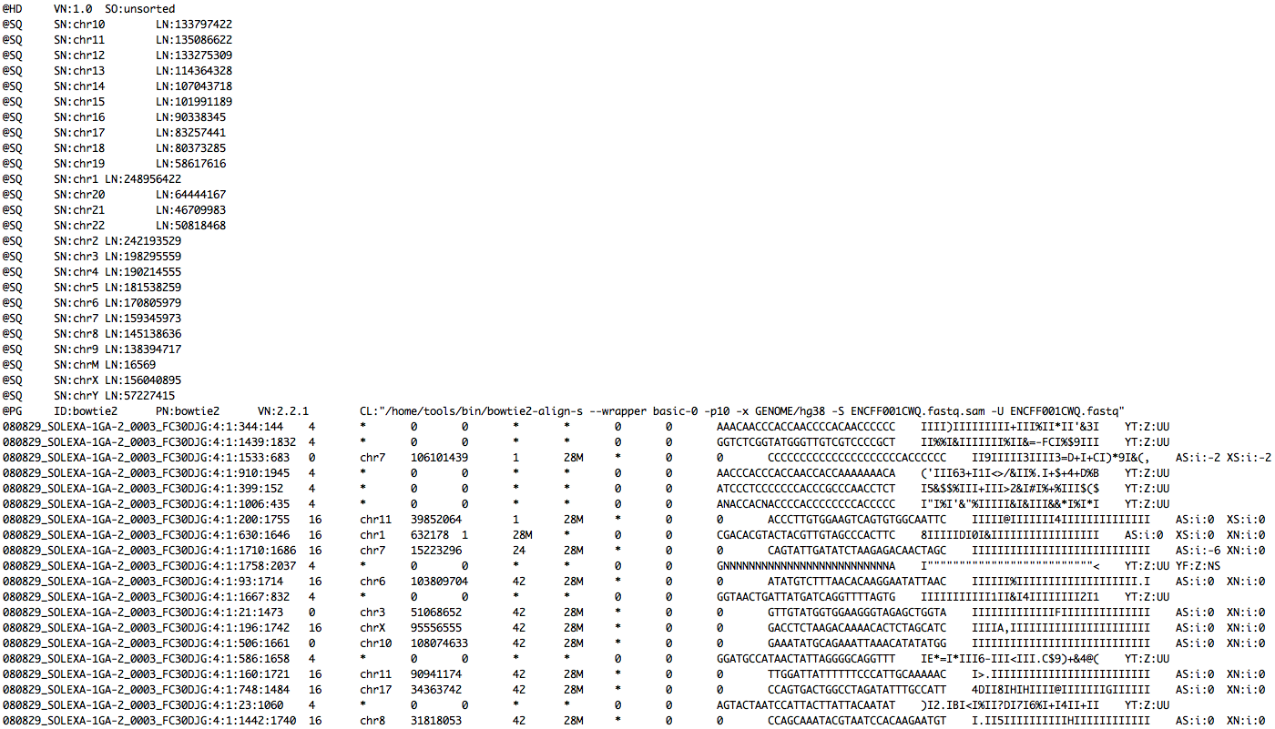
(SAM format specification: https://samtools.github.io/hts-specs/SAMv1.pdf) - SAM is a TSV file with header, BAM is its compressed binary version. The columns are:
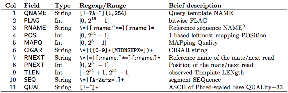
Read mapping example
FASTQ
+ indexed database

-> SAM file
Samtools example
(Manual: http://www.htslib.org/doc/samtools.html)
- A toolkit designed for SAM/BAM manipulations
- View:
- Statistics assessment:
- Format conversion:
- Filtering:
samtools view file.samsamtools view -F 4 input.sam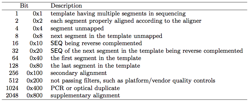
samtools stats file.samsamtools view -b file.sam > file.bamBedtools example
(Manual: https://bedtools.readthedocs.io/en/latest/content/bedtools-suite.html
BED format specification: https://genome.ucsc.edu/FAQ/FAQformat.html)
- A toolkit for conversion and manipulations with BED:
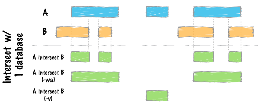
- A powerful tool for genomic arithmetics:
(Tutorial: https://bedtools.readthedocs.io/en/latest/)
bedtools bamtobed -i file.bam > file.bed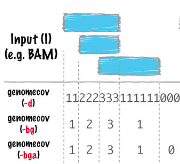
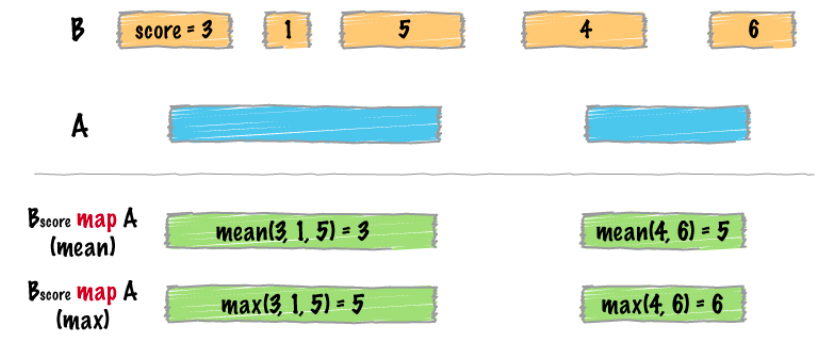
map
intersect
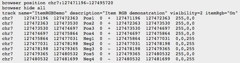
Other formats
- BED
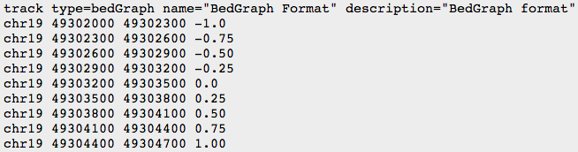
- BEDGRAPH
- BIGWIG: binary compressed format, created with UCSC tools (see below)
UCSC genome browser & UCSC tools
- UCSC maintains genome browser and has a set of tools: https://genome-euro.ucsc.edu/

UCSC tools example
Full set of compiled tools: http://hgdownload.soe.ucsc.edu/admin/exe/linux.x86_64/
- We will need file conversion, check the documentation:
bedGraphToBigWig -hNext step: index build and mapping
These steps are time-consuming, but we have to complete them:
- Build genome index with name prefix hg38_chr5-6_index:
- Run mapping of your FASTQ file for the index hg38_chr5-6_index:
cd GENOME/
bowtie2-build dm6.fa
bowtie2-build -hbowtie2 -hbowtie2 --very-sensitive -x ./GENOME/dm6 <file.fastq> -S <file.sam>less <file.sam>ls
cd ../Don't run this code, it's FYI
Filtering
- Filter only uniquely mapped reads with high alignment score, sort resulting file:
samtools view -h -F 4 <file.sam> | lesssamtools --helpsamtools view -h -q 10 <file.sam> > <file_filtered.sam>samtools view -b -q 10 <file.sam> > <file_filtered.bam>
samtools sort <file_filtered.bam> > <file_filtered.sorted.bam>Don't run this code, it's FYI
File format conversion
- Read the documentation of bedtools:
- Convert BAM to BEDGRAPH genome coverage:
- Create files with genomic windows (1Kbp bin size, don't forget to use your chromosome!). Convert BAM to BEDGRAPH coverage of windows:
bedtools makewindows -g GENOME/chrom_sizes.tsv -w 1000 > hg38_windows.1000.bed
grep "chr5" hg38_windows.1000.bed > chr5_windows.1000.bed
bedtools genomecov -ibam <file_filtered.sorted.bam> -bga -split > <file.genomecov.bedgraph>bedtools genomecov -h
bedtools makewindows -h
bedtools coverage -h
bedtools coverage -counts -a chr5_windows.1000.bed -b <file_filtered.sorted.bam> > <file.binned.bedgraph>- Check the resulting files, you should see genome coverage
files (*.genomecov.*) and binned datasets (*.binned.*):
ls
less <file.genomecov.bedgraph>
less <file.binned.bedgraph>
Don't run this code, it's FYI
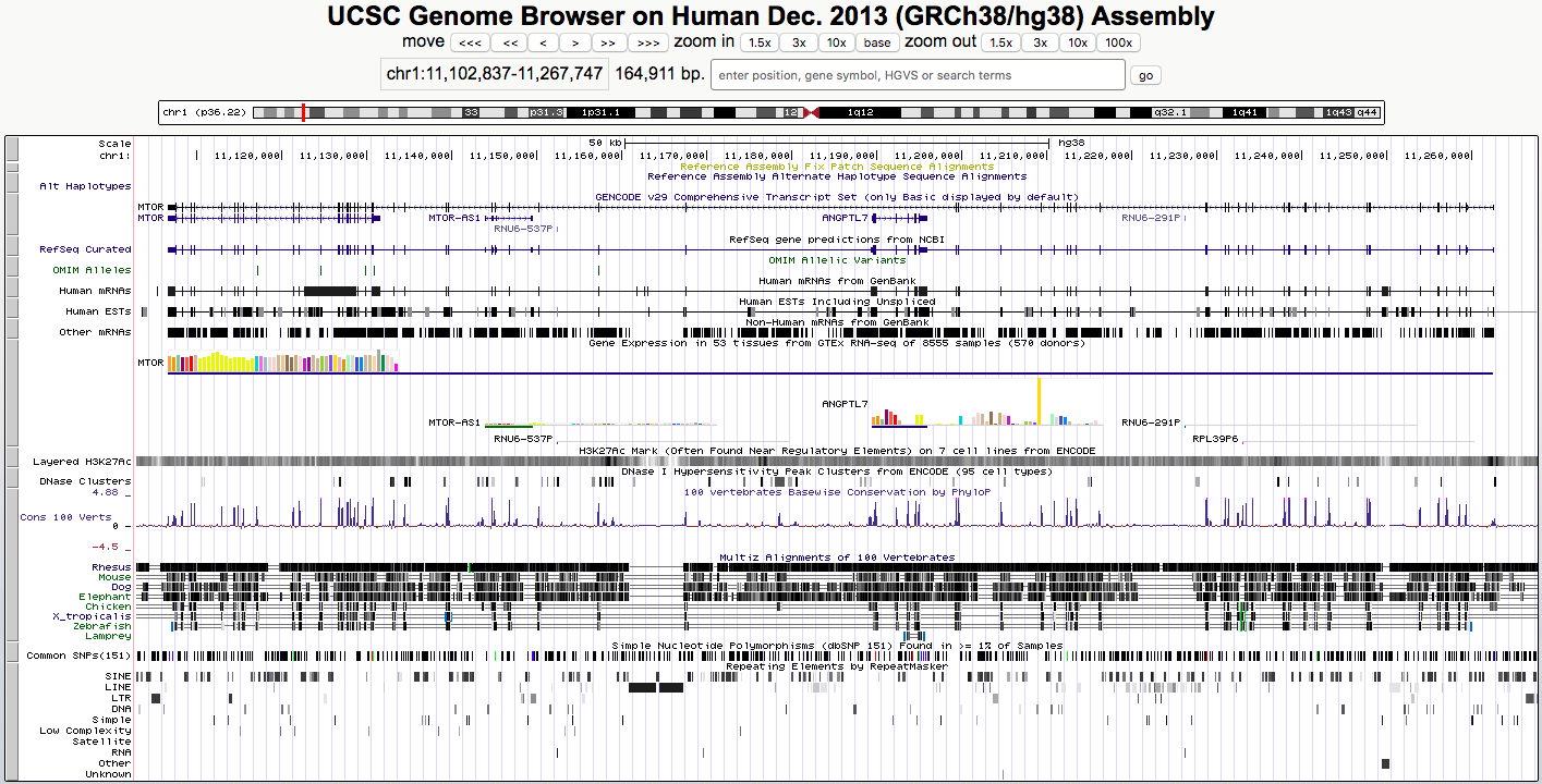
BEDGRAPH tracks visualization
We will use UCSC browser for bedgraph files visualization.
- Download both files file.genomecov.bedgraph and file.binned.bedgraph to your local computer.
- Manually add the header to your file:
(see UCSC recommendations: https://genome.ucsc.edu/goldenPath/help/bedgraph.html)
track type=bedGraph visibility=full
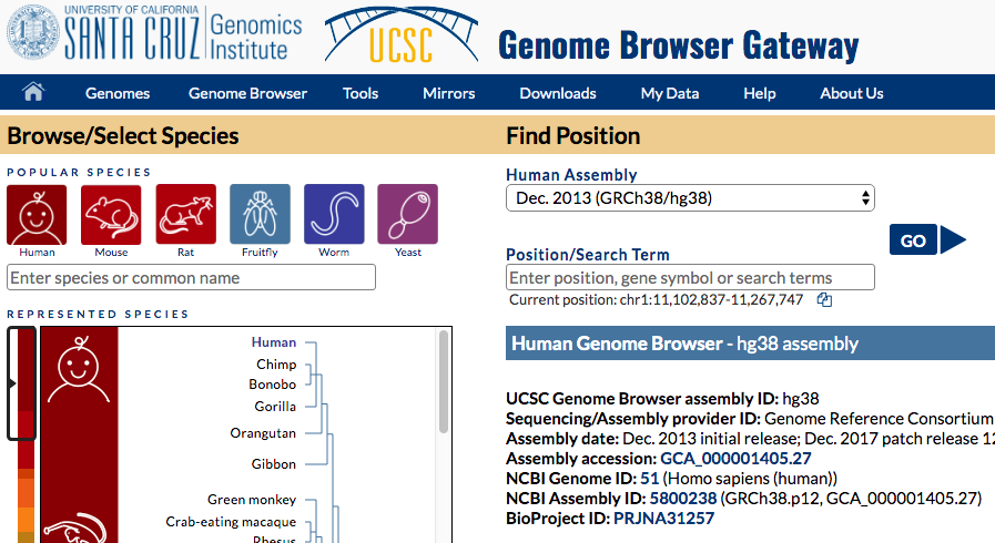
- Go to UCSC genome browser, hg38 genome:
https://genome-euro.ucsc.edu/cgi-bin/hgTracks?db=hg38
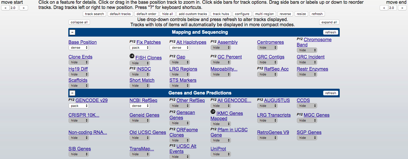
UCSC genome browser
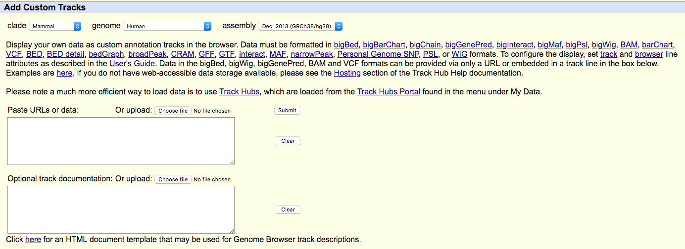
- Find "add custom tracks button".
- Check the upload form:
- Upload your modified BEDGRAPH files (with headers) to UCSC ("Choose file" -> "Submit").
Experiments comparison
- Convert BEDGRAPH to BIGWIG:
- Rename your final file (substitute YOUR_CELL_LINE and CHROMOSOME):
- Find three of your colleagues with the same chromosome as you. Exchange your BIGWIG files and upload them to the server. Thus you should collect at least 4 BIGWIG files with recognisable names (cell line and chromosome should be present in the file names).
mv <file.genomecov.bw> <YOUR_CELL_LINE-CHROMOSOME.bw>bedGraphToBigWig <file.genomecov.bedgraph> ./GENOME/chrom_sizes.tsv <file.genomecov.bw>Samples comparison
Task 1 (1 point): Provide the final set of commands that you've used and briefly justify the parameters.
Task 2 (1 point): Report the final scatteplot for 100 Kb. Describe your observations.
Task 3 (*1 point): Repeat the procedure for 10 Kb and 1 Kb and report the changes in observations. At what resolution you might observe the differential DNase I signal?
- Collect at least 4 DNase I results for your chromosome in bigWig format. One of them should be yours, the others you may take from /home/shared/EpiPract1/. you may use conda environment "hic" (see instructions on activation can be found in EpiPract3).
- Use multiBigwigSummary to create a summary file. Use bins mode, bin size 100 Kb:
- Plot correlations obtained from your file as a scatterplot:
- Try to adjust the parameters of the plot to improve the analysis. Try plotting in log-scale (--log1p). If you get the warning about the outliers, try to fix it: use --removeOutliers and --corMethod spearman. Which method worked?
- * Repeat the procedure for 10 Kb and 1 Kb. You may want to create another intermediary summary file for that. Inspect the changes.
multiBigwigSummary bins --binSize 100000 -b ${file1.bw} ${file2.bw} ${file3.bw} ${file4.bw} -o ${summary.npz}plotCorrelation -in ${summary.npz} --corMethod pearson --skipZeros --whatToPlot scatterplot -o ${scatterplot.png}Experiments comparison
6. Plot correlations for 100 Kb as a heatmap. Use the parameters that you found to be representative for the scatterplots. For example:
7. Inspect and describe your observations. Adjust the visualization, if needed.
plotCorrelation -in ${summary.npz} --corMethod pearson --skipZeros --whatToPlot heatmap --colorMap RdYlBu --plotNumbers -o ${heatmap.png}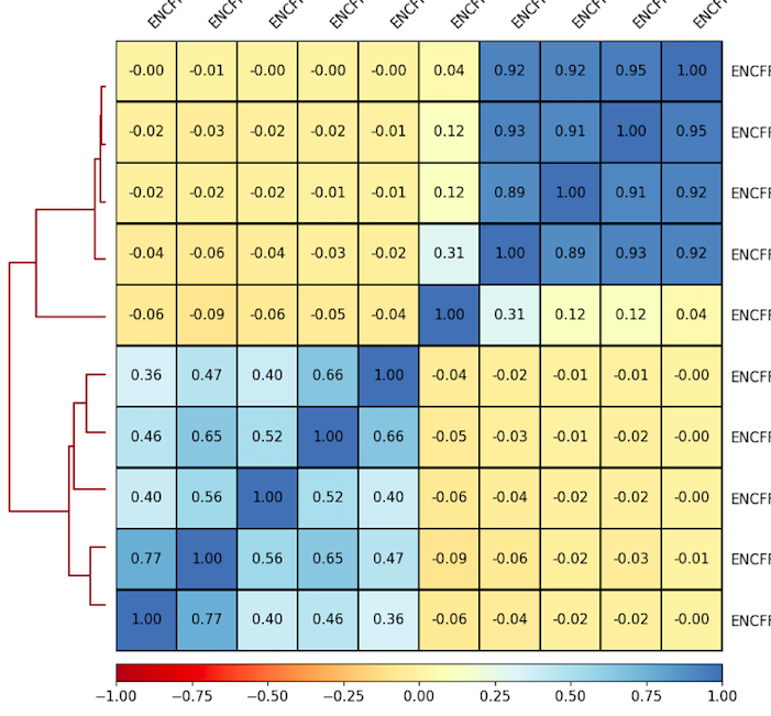
Result of clustering
Correlation coefficient
Labels are not representative
(correct if needed)
Practical Part: Enrichment Profiles
We will:
- Call TADs in S2 cell line (Wang et al. 2017),
- Plot the enrichment profiles for multiple factors.
We'll need conda environment "hic" (see instructions on activation can be found in EpiPract3).