Spatial structure of chromatin:
introduction to Hi-C
Aleksandra Galitsyna
“Analysis of omics data” course
Skoltech Term 4
24 April 2020

This presentation can be found at https://slides.com/agalicina/epigenetics-practice3-2020
Chromatin spatial structure
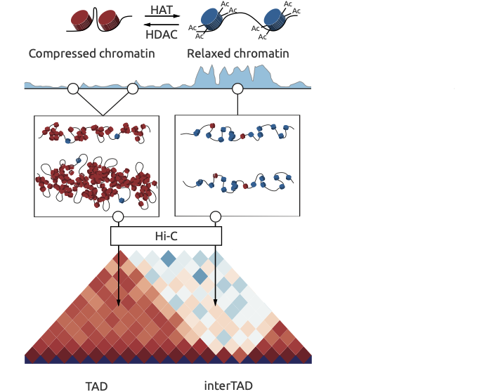
Ulianov et al. Genome Biology 2016

Methods to study chromatin structure
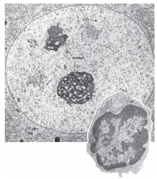
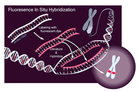
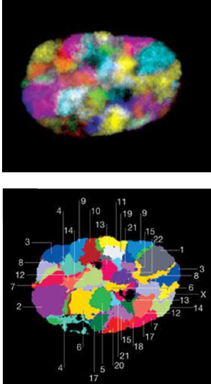
Microscopy:
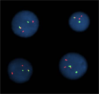
Microscopy with fluorescing marks:
(FISH)
For 2 marks:
For multiple marks:
Chromatin conformation capture
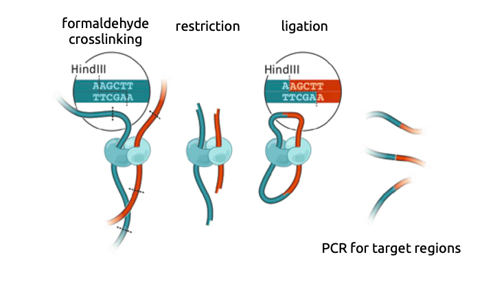
3C: Dekker et al. Science 2002
Hi-C
Viewpoint
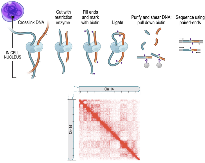
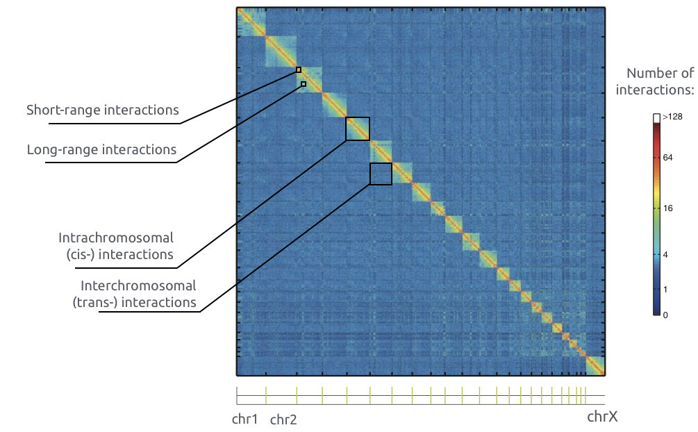
High-throughput chromosomes conformation capture:
DNA interactome map:
Lieberman-Aiden et al. Science 2009
Variety of C-based techniques

Adopted from Schmitt Nature Reviews 2016
Chromatin spatial structure
Adopted from Imakaev et al. Nature Methods 2012
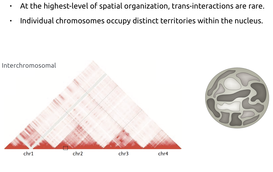
Chromosome territories
Bonev et al. Nature Reviews 2016
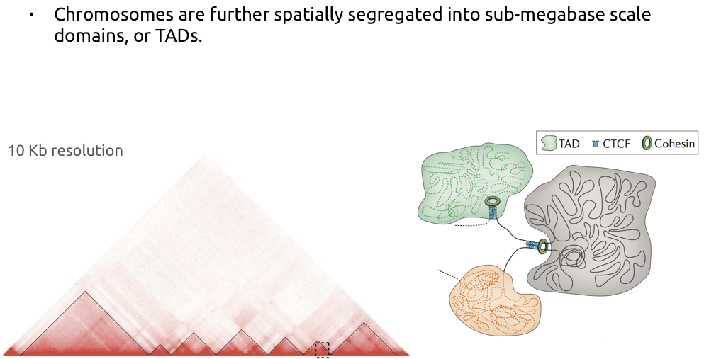
TADs
Bonev et al. Nature Reviews 2016
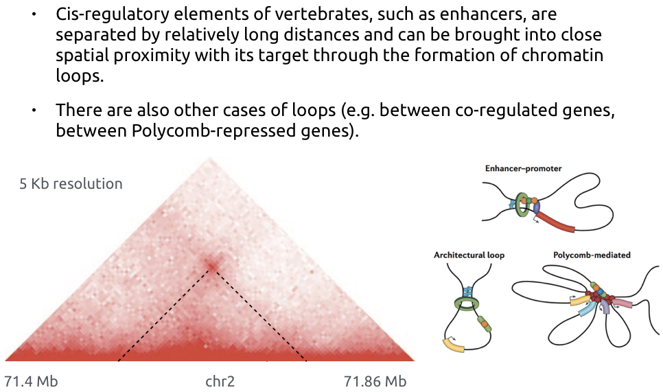
Loops of chromatin
Bonev et al. Nature Reviews 2016
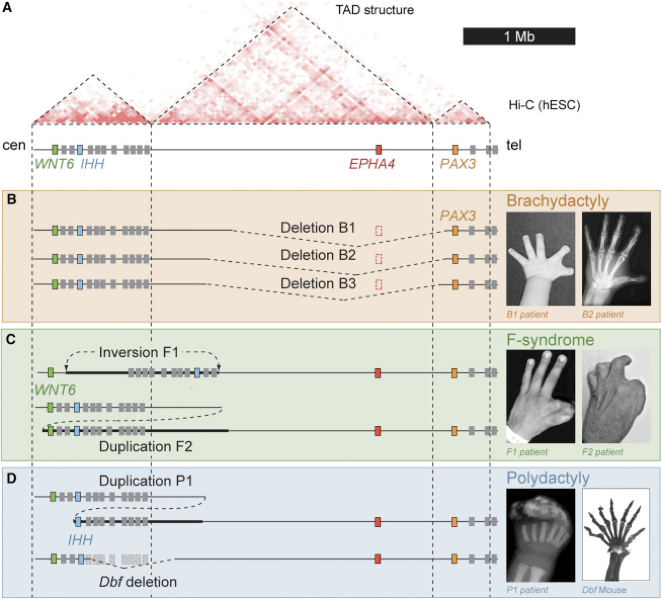
The importance of TADs and loops
Lupiáñez et al., Cell, 2015

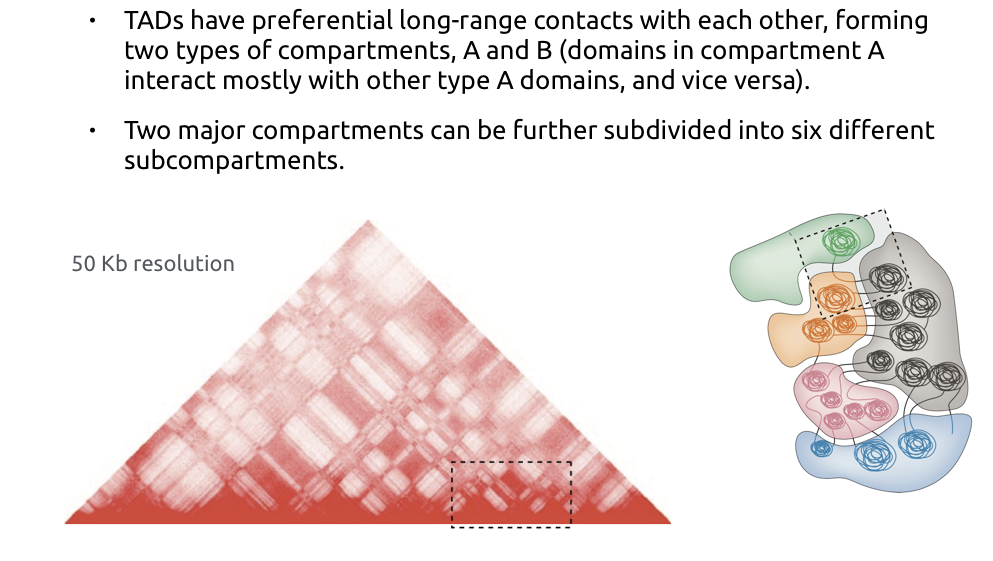
Compartments of chromatin
Bonev et al. Nature Reviews 2016
Hi-C data processing outline
1. Reads mapping
- File with mapping position of pairs
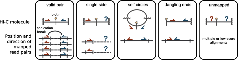
2. Contacts filtration
- Removal of PCR duplicates
- Filtering by restriction fragments
3. Contacts map retrieval
- Binning
4. Balancing and map normalization
5. Features calling (TADs, compartments, loops)
Chromatin spatial structure
Adopted from Lajoie et al., The Hitchhiker's guide to Hi-C analysis: Practical guidelines.
Methods 2015
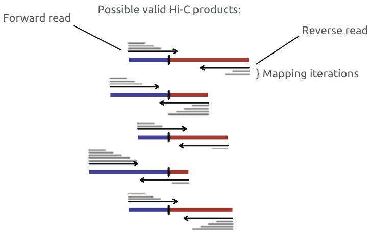
Iterative mapping or mapping allowing chimeric reads (split read alignment, e.g. bwa mem)
Chromatin spatial structure
Imakaev et al. Nature Methods 2012
Chromatin spatial structure
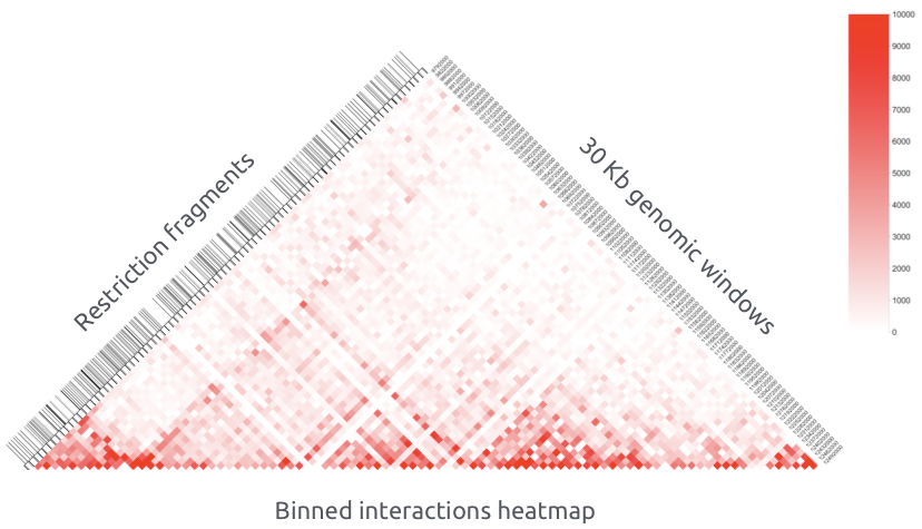
Hi-C restriction fragments are assigned to bins (sequential same size genomic windows) and aggregated by taking the sum:
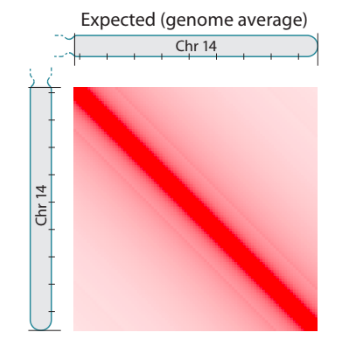
Hi-C data correction
Two major types of approaches:

Adopted from Schmitt et al. Nature Reviews 2016
Hi-C data correction
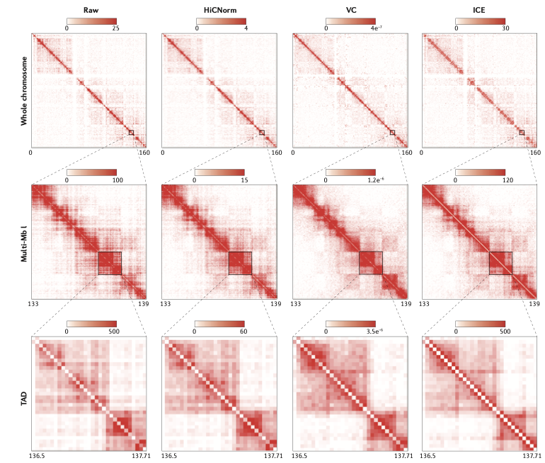
Schmitt et al. Nature Reviews 2016
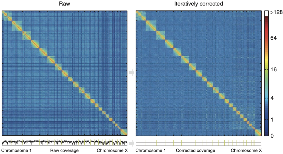
Iterative correction
Imakaev et al. Nature Methods 2012
Hi-C data mapping
Forcato et al. Nature Methods 2017

There are various tools for Hi-C data processing:
Example of Hi-C data processing
1. Mapping
- Tools : bwa, samtools
- Output: bam file
2. Filtering, sorting, creation of the contacts list
- Tools: pairtools
- Output: pairs file
3. Binning and normalization
- Tools: cooler
- Output: cool file
4. Aggregation
- Tools: cooler
Output: multires.cool (mcool) file
Hi-C data processing
All of the processing steps are accessible in the form of pipelines,
e.g. distiller-nf:
https://github.com/mirnylab/distiller-nf

Practice:
Mapping Hi-C data
Practice results
- As a result of this practice I expect a small report on the results (free form, PDF format).
- The questions that should be covered in the report are highlighted in red.
- Your mark for the report cannot exceed 10 points.
- The deadline is in a week (next Friday).
Adjust the environment
1. Login to the server via terminal:
or use Putty on Windows.
(example instructions https://www.ssh.com/ssh/putty/windows/#sec-Configuration-options-and-saved-profiles)
2. Create the folder with your project:
3. Activate prepared environment:
(if you have problems with it, please, contact the TA)
4. Check your environment:
ssh username@servernamemkdir EpiPract3
cd EpiPract3export PATH="/home/galitsyna/anaconda3/bin:$PATH"
conda activate hicls # Should list all the filesin the directory
pwd # Should result in your currentl location
conda list # Should list all the programs installed, if conda imported successfully.Get the data
- Copy to the local folder:
- Check the content and file sizes:
$ cp /home/galitsyna/EpiPract3/fastq/your_file.fa.gz ~/EpiPract3/
$ mkdir ~/EpiPract3/genome/
$ cp /home/galitsyna/EpiPract3/genome/* ~/EpiPract3/genome/
$ ls -hts
$ ls -hts genome/| Name | Files for EpiPract3 | |
|---|---|---|
| Anastasia Pivnyuk | nuclear_cycle_12_repl_1_run1_1.fastq.gz | nuclear_cycle_12_repl_1_run1_2.fastq.gz |
| Nikita Sharaev | nuclear_cycle_12_repl_1_run2_1.fastq.gz | nuclear_cycle_12_repl_1_run2_2.fastq.gz |
| Artemy Shumskiy | nuclear_cycle_12_repl_1_run3_1.fastq.gz | nuclear_cycle_12_repl_1_run3_2.fastq.gz |
| Dmitrii Kriukov | nuclear_cycle_12_repl_1_run4_1.fastq.gz | nuclear_cycle_12_repl_1_run4_2.fastq.gz |
| Pletenev Ilya | nuclear_cycle_12_repl_2_run1_1.fastq.gz | nuclear_cycle_12_repl_2_run1_2.fastq.gz |
| Konstantin Chernyshov | nuclear_cycle_12_repl_2_run2_1.fastq.gz | nuclear_cycle_12_repl_2_run2_2.fastq.gz |
| Ivan Kuznetsov | nuclear_cycle_13_repl_1_run1_1.fastq.gz | nuclear_cycle_13_repl_1_run1_2.fastq.gz |
| Anna Kalinina | nuclear_cycle_13_repl_1_run2_1.fastq.gz | nuclear_cycle_13_repl_1_run2_2.fastq.gz |
| Sofya Kasatskaya | nuclear_cycle_13_repl_1_run3_1.fastq.gz | nuclear_cycle_13_repl_1_run3_2.fastq.gz |
| Julia Bocharkina | nuclear_cycle_12_repl_2_run1_1.fastq.gz | nuclear_cycle_12_repl_2_run1_2.fastq.gz |
| Vasily Borodin | nuclear_cycle_14_repl_1_run1_1.fastq.gz | nuclear_cycle_14_repl_1_run1_2.fastq.gz |
| Sofia Kamalyan | nuclear_cycle_14_repl_1_run2_1.fastq.gz | nuclear_cycle_14_repl_1_run2_2.fastq.gz |
| Anna Krasivskaya | nuclear_cycle_14_repl_1_run3_1.fastq.gz | nuclear_cycle_14_repl_1_run3_2.fastq.gz |
| Aleksandra Ozerova | nuclear_cycle_14_repl_1_run4_1.fastq.gz | nuclear_cycle_14_repl_1_run4_2.fastq.gz |
| Victoria Kobets | 3-4h_repl_1_run1_1.fastq.gz | 3-4h_repl_1_run1_2.fastq.gz |
| Slesareva Anastasiia | 3-4h_repl_1_run2_1.fastq.gz | 3-4h_repl_1_run2_2.fastq.gz |
| Mikhail Moldovan | 3-4h_repl_1_run3_1.fastq.gz | 3-4h_repl_1_run3_2.fastq.gz |
| Viktor Mamontov | 3-4h_repl_1_run4_1.fastq.gz | 3-4h_repl_1_run4_2.fastq.gz |
| Evgeniia Alekseeva | 3-4h_repl_2_run1_1.fastq.gz | 3-4h_repl_2_run1_2.fastq.gz |
| Trofimova Anna | 3-4h_repl_2_run2_1.fastq.gz | 3-4h_repl_2_run2_2.fastq.gz |
The files that should be in the genome folder:
- dm3.fa.gz - File with Drosophila genome sequence, dm3 assembly
- dm3.fa.gz.amb
- dm3.fa.gz.ann
- dm3.fa.gz.bwt
- dm3.fa.gz.pac
- dm3.fa.gz.sa
- dm3.reduced.chrom.sizes - File with chromosome sizes for Drosophila genome
The files that should be in you working directory:
- <Your unique name>_1.fastq.gz
- <Your unique name>_2.fastq.gz
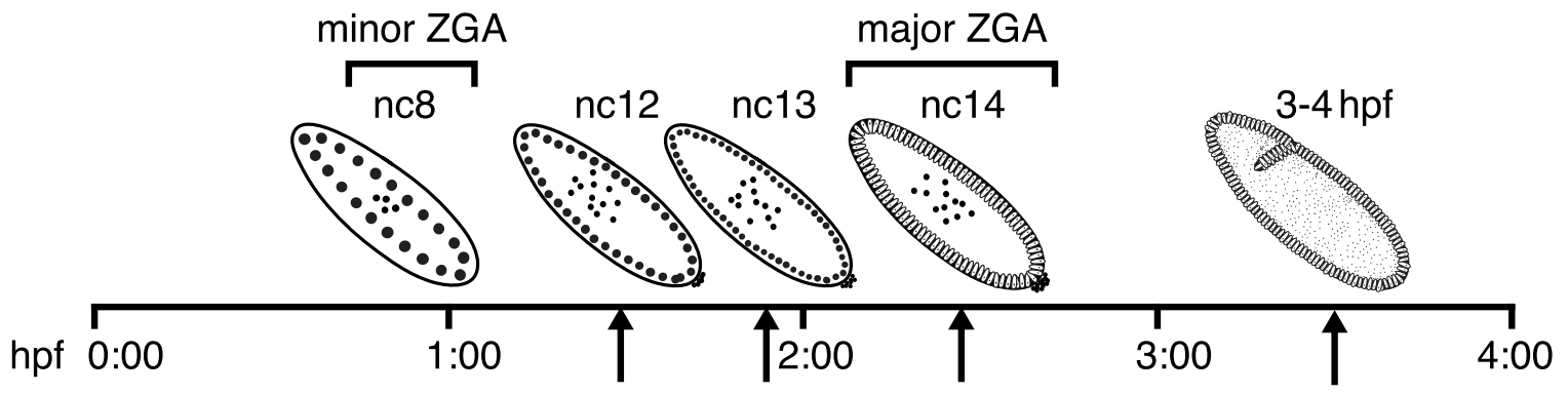
What's in the data?
- We will analyse the data from the paper on Drosophila melanogaster embryogenesis:
Hug et al. Cell 2017 - We have several data points and Hi-C for them (you all have different replicates of them):
- I suggest you not to look to the results of the paper until you don't get the pictures of your maps at 20 Kb resolution.
Map Hi-C data
- Map FASTQ -> BAM:
$ bwa mem -t 1 -v 3 -SP ${genome_file.fa.gz} ${fastq_file1} ${fastq_file2} > ${output.sam}
$ samtools view -bS ${output.sam} > ${output.bam}
$ pairtools parse --walks-policy 5unique -c ${chromosome_sizes} ${input.bam} -o ${output.pair}
$ pairtools dedup --output-stats ${output.stats} ${output.pair} -o ${output.nodup.pair}$ cooler cload pairs -c1 2 -c2 4 -p1 3 -p2 5 ${chromsizes}:20000 ${input.nodup.pair} ${output.cool}Task 1 (1 point): Report the number of uniquely mapped pairs, number and fraction removed after deduplication.
Task 2 (2 points): Visualize the data with cooler show in png format for any genomic region of 2 Mb size before and after correction. Report the resulting figures and your observations.
- Parse BAM -> PAIR file and remove PCR duplicates:
- Load cooler map (at 20 Kb resolution, note the ":2000"):
$ cooler balance ${input.cool}- Balance it:
Scaling plots
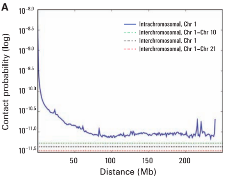
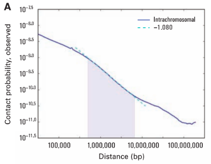
Lieberman-Aiden, 2009
Scaling plots
Task 3 (optional*): Convert your cool file to h5 with HiCExplorer command hicConvertFormat. Run hicInfo on the resulting file. What are the differences from cooler info?
Task 4 (optional*): Create the scaling plot for your dataset with HiCPlotDistVsCounts. What are your observations?
We'll try to plot our own scaling plots on the data with HiCExplorer.
Expected results of the report
5 points in total (rescaled proportionally to 10 in Canvas):
- 1 point for the running the initial steps of the script
- 2 points for finishing the pipeline and visualizing the result with and without iterative correction.
- 2 points for the part on genome reassembly (not included in this presentation).
Optional tasks (about HiCExplorer can substitute the points that you might miss in the required part).