Topic Definition

Topic Definition

Multiple Linear Regression with Interactions and Dummy Variables

Linear Regression

Multiple

Dummy Variables

Interactions

Response is

a linear transformation

of the predictor.

Response is

a linear combination

of several predictors.

Response is

a linear combination

of several predictors,

some being binary.

Response is

a linear combination

and products

of several predictors,

some being binary.

Multiple Linear Regression with Interactions and Dummy Variables,
target audience is class of first semester statistics students
at the basic level.

Do not discuss optimization.

Only simple statistics/metrics

PISA x Socio-economics and Climate?

Setting

X

Predictor / Explanatory Variables

Y

Response / Outcome (Observation)

Ŷ

Prediction

y-ŷ

Residual

R2

R-square = square of Pearson correlation ρ

\dfrac{ (\sum_i x_i y_i) }{ \sqrt{ (\sum_i x_i^2) (\sum_i y_i^2) } }

ρ

Pearson correlation

Data and Problem

Hypthesis:

The MATH PISA score (2022) per country can be explained by social, environmental and economical variables

The Programme for International Student Assessment (PISA) is the Organisation for Economic Co-operation and Development's (OECD) programme measuring 15-year-olds’ ability to use their reading, mathematics and science knowledge and skills to meet real-life challenges.

https://www.oecd.org/en/about/programmes/pisa.html

Linear Regression

Variables:

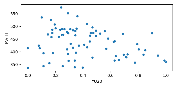
MATH: PISA (2022) score of 79 countries

YU20: Youth Unemployment rate in ~2020 (WorldBank)

Linear Regression?

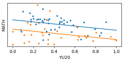
MATH ~ YU20

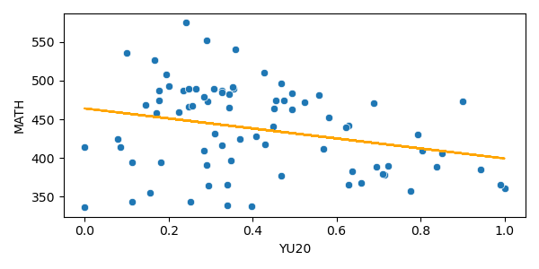
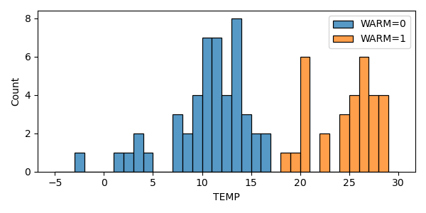
WARM {0,1}: average yearly temperature ≥ 18°C (WorldBank)

Not so good

What if we add another variable?

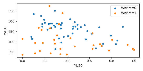
Interaction and Dummy Variable

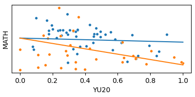
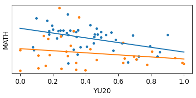
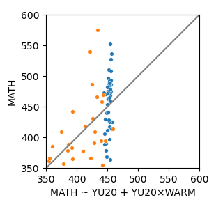
Model 2: Interaction

MATH ~ YU20 + YU20×WARM

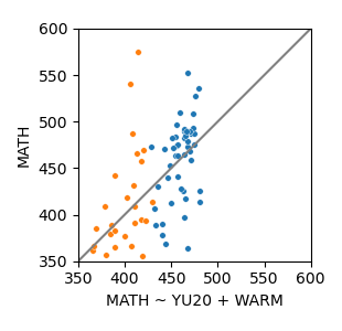
Model 1: Dummy Variable

MATH ~ YU20 + WARM

Model 3: Both

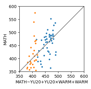
MATH ~ YU20 + YU20×WARM + WARM

Same slope
Different intercepts

Dummy Variable

Different slopes
Same intercept

Model Selection

\begin{split} \frac{1}{n}SSR &= 795.6 \\ R^2 &= 0.751 \\ \mathrm{adj.}R^2 &= 0.730\\ \mathrm{AIC}&=765.8\\ \mathrm{BIC}&=782.4\\ \end{split}

\begin{split} \frac{1}{n}SSR &= 2146.0 \\ R^2 &= 0.327 \\ \mathrm{adj.}R^2 &= 0.301\\ \mathrm{AIC}&=838.2\\ \mathrm{BIC}&=847.7\\ \end{split}

↑: accounting for
the number of predictors

\mathrm{adj.}R^2

\mathrm{AIC\: BIC}

↓:
Akaike/Bayesian
Information Criteria

↑: proportion of the variance explained

R^2

↓: sum of squared residuals

SSR

Model Selection

==============================================================================
                 coef    std err          t      P>|t|      [0.025      0.975]
------------------------------------------------------------------------------
Intercept    497.3029     15.255     32.599      0.000     466.913     527.693
YU20         -91.1878     33.065     -2.758      0.007    -157.057     -25.318
WARM         -78.0385     21.575     -3.617      0.001    -121.017     -35.060
YU20:WARM     51.3942     44.789      1.147      0.255     -37.831     140.619

==============================================================================
                 coef    std err          t      P>|t|      [0.025      0.975]
------------------------------------------------------------------------------
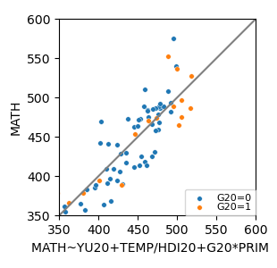
Intercept    472.2815     12.770     36.984      0.000     446.825     497.738
YU20         -55.1106     14.126     -3.901      0.000     -83.270     -26.952
TEMP         -19.5058      1.660    -11.749      0.000     -22.815     -16.196
TEMP:HDI20    21.4286      2.106     10.176      0.000      17.231      25.626
G20          117.0291     33.314      3.513      0.001      50.619     183.439
PRIM          46.7952     21.065      2.221      0.029       4.802      88.788
G20:PRIM    -252.5079     76.412     -3.305      0.001    -404.833    -100.182

MATH ~ YU20 + YU20×WARM + WARM

MATH ~ YU20 + TEMP + TEMP×HDI20 + G20 + G20×PRIM + PRIM

Summary

Summary

Multiple Linear Regression with interactions and dummy variables:

It is a linear regression with more than one predictor, including binary ones, and products between predictors.

Model Selection:

Pay attention to the p-values of the coefficients.

Favor low SSR, high adjusted R2, low AIC/BIC.

Favor homoscedastic and normally distributed residuals.

Remark:

The regressed lines do not always match that of stratified models (one model per dummy combination).

Linear Regression

Linear Regression

Model:

\operatorname{MATH} = \beta_0 + \beta_1 \times \operatorname{YU20} + \varepsilon

\beta_0 = 464.13 \quad \beta_1 = - 64.68

Linear Regression

Model Selection:

R^2 = \frac{ \sum_i \hat{y}_i - \bar{y} } { \sum_i y_i - \bar{y} } \in [0,1]

Proportion of the variance
in MATH predicted by YU20.

Higher is better.

R^2 = 0.075

SE = \sqrt{ \frac{ \sum_i (y_i -\hat{y}_i)^2 } { n-2 } }

Standard Error measures the average deviation to the regression line.

Lower is better.

SE = 55.018

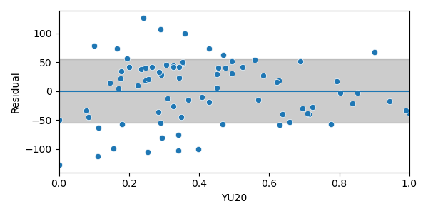
Independent from each other;
Homoscedastic, (variance indep. of YE20);
Normally distributed (low skewness ).

\gamma_1 = \frac{ \frac{1}{n} \sum_i (r_i - \bar{r})^3 } { \Big( \frac{1}{n} \sum_i (r_i - \bar{r})^2 \Big)^{3/2} }

\text{where } r_i = y_i - \hat{y}_i

\gamma_1

\gamma_1 = -0.232

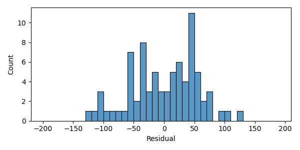
Residuals should be:

Not very satisfying...

Data and Problem

Variables:

MATH: average PISA2022 score of 79 countries

YU20: Youth Unemployment rate in ~2020 (WorldBank)