Chapter 7: Evaluating, comparing, and expanding models
presentation for the INM-6 bookclub
30 Aug 2019
presenter: Alexandre René
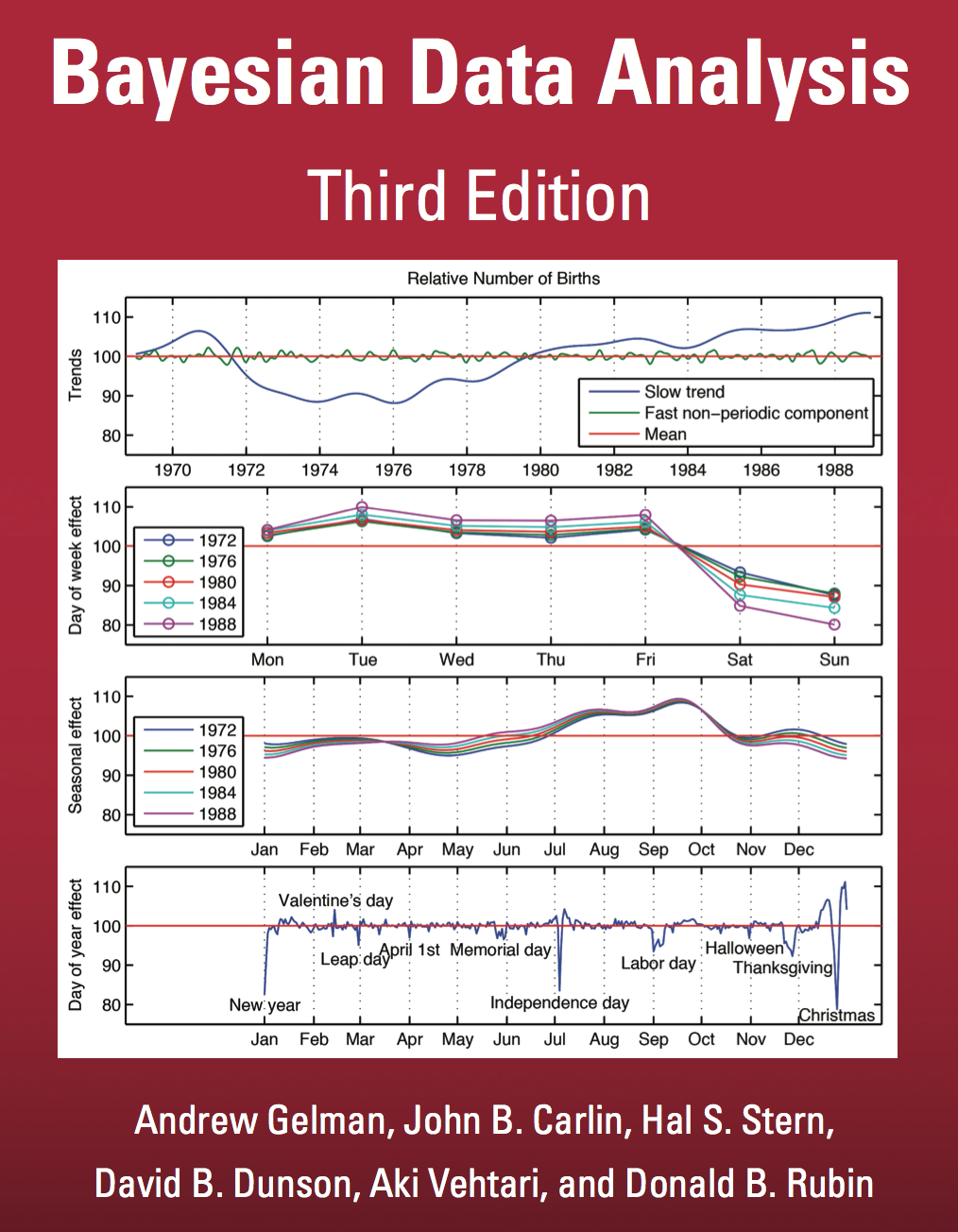
Bayesian Data Analysis
“Inference is normal science.
Model-checking is revolutionary science.”
– Andrew Gelman
Why this chapter
- Not Bayesian 101
- Still among “basic Bayesian methods”
- Seemed more interesting than Chap 6 :-P
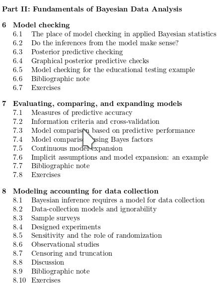
7 Evaluating, comparing, and expanding models
7.
- Measures of predictive accuracy
- Information criteria and cross-validation
- Model comparison based on predictive performance
- Model comparision using Bayes factors
- Continuous model expansion
- Implicit assumptions and model expansion: an example
- Bibliographic note
- Exercises
7.
7.
7.
7.
7.
7.
7.
7.1 Measures of predictive accuracy
observed data: \(y\)
new data: \(\tilde{y}_i\)
parameters: \(θ\)
point estimate: \(\hat{θ}\)
likelihood: \(p(y|θ) \)
true model: \(f(y)\)
prior: \(p(θ)\)
posterior: \(p_{\text{post}}(θ) = p(θ|y)\)
posterior predictive distribution:
7.1 Measures of predictive accuracy
lpd
Log predictive density,
aka log-likelihood
elpd
expected log predictive density for a new data point
replace \(f\), \(θ\) by an estimate (e.g. \(p_{\text{post}}\), \(\hat{θ}\))
plug-in estimate
Approximations
Non-computable measures we want to use
lppd
log pointwise (posterior) predictive density
Needs true \(θ\)
Needs true \(f\)
Uses sample data \(y\)
elpd|\(\hat{θ}\)
expected log predictive density, given \(\hat{θ}\)
Log predictive density scoring rule (Log-likelihood)
Scoring rule: Measure of predictive accuracy for probabilistic prediction. Good scoring rules are proper and local
- proper: \(\text{argmax}(\text{score}|θ)\) returns \(θ\)
- local: some \(\tilde{y}\) are more important than others
It can be shown that the logarithmic score is the unique (up to an affine transformation) local and proper scoring rule, and it is commonly used for evaluating probabilistic predictions.
The advantage of using a pointwise measure, rather than working with the joint posterior predictive distribution, ppost() is in the connection of the pointwise calculation to cross-validation
Regarding the use of LPD as a model score:
Given that we are working with the log predictive density, the question may arise: why not use the log posterior? Why only use the data model and not the prior density in this calculation? The answer is that we are interested here in summarizing the fit of model to data, and for this purpose the prior is relevant in estimating the parameters but not in assessing a model’s accuracy.
7.2 Information criteria and cross-validation
- Measures of predictive accuracy are called information criteria.
- They are usually expressed in terms of the deviance, defined as \(-2 \log p(y|\hat{θ})\).
- Basic idea: we want to use lppd, but to compare different models we need to consider effective parameters.
Why effective parameters matter
Assume \(\dim θ = k\) and \(p(θ|y) \to \mathcal{N}(θ_0, V_0/n)\) as \(n \to \infty\). Then
\(\sum_1^k \mathcal{N}(0,1)\)
So
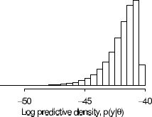
Fig 7.2
max lpd: -40.3
mean lpd: -42.0
no. params: 3
\({}^-40.3 - {}^-42.0 = 1.7 \approx k /2\)
I.e. the 3 parameters are expected to contribute a factor \(k\) to the deviance
Estimating out-of-sample predictive accuracy using available data
-
Within-sample predictive accuracy
Ignore the bias. -
Akaike information criterion (AIC)
Subtract \(k\) from deviance. -
Deviance information criterion (DIC)
Replace \(k\) with Bayesian estimate for effective number of parameters.
We know of no approximation that works in general, but predictive accuracy is important enough that it is still worth trying.
(Estimating lpd or elpd)
Basic idea: start from lppd and correct for bias due to parameters.
-
Watanabe-Akaike (widely available) information criterion (WAIC)
Fully Bayesian information criterion. Averages over posterior. -
Leave-one-out cross-validation (LOO-CV)
Evaluate lppd on the left-out data. Bias usually neglected.
Example: WAIC
Effective number of parameters:
Then
The authors also define an \(p_{\text{WAIC}_2}\).
the accuracy of a fitted model’s predictions of future data will generally be lower, in expectation, than the accuracy of the same model’s predictions for observed data
Effective number of parameters as a random variable
[C]onsider the model \(y_i, \dotsc, y_n \sim N(θ, 1)\), with \(n\) large and \(θ \sim U(0, ∞)\). If the measurement \(y\) is close to zero, then \(p \approx 1/2\), since roughly half the information in the posterior distribution is coming from the prior constraint of positivity. However if \(y > 0\) is large, the effective number of parameters is 1.
Informative prior distributions and hierarchichal structures tend to reduce the amount of overfitting
7.3 Model comparison based on predictive performance
For both nested and nonnested models important to adjust for overfitting, especially when complexities strongly differ.
Illustrated on 8-schools model:
| School | yⱼ | σⱼ |
|---|---|---|
| A | 28 | 15 |
| B | 8 | 10 |
| C | -3 | 16 |
| D | 7 | 11 |
| E | -1 | 9 |
| F | 1 | 11 |
| G | 18 | 10 |
| H | 12 | 18 |
No pooling model
\(p = 8\)
Complete pooling model
\(p = 1\)
Hierarchichal model
\(1 \leq p \leq 8\)
Table 5.2
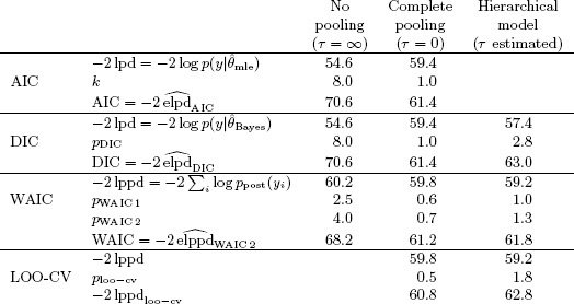
7.3 Model comparison based on predictive performance
Table 7.1
Evaluating predictive error comparisons
Two issues: “statistical” and “practical” significance.
- Rule of thumb for nested models:
\(Δ > 1 \Rightarrow \text{statistically significant}\). - For practical significance:
- Use expert knowledge.
- Calibrate with smaller models.
Out-of-sample prediction error also does not tell the whole story: Substantial improvements may be small on an absolute scale.
Bias induced by model selection
If the number of compared models is small, the bias is small, but if the number of candidate models is very large (for example, if the number of models grows exponentially as the number of observations n grows) a model selection procedure can strongly overfit the data. […] This is one reason we view cross-validation and information criteria as an approach for understanding fitted models rather than for choosing among them.
Thus we see the value of the methods described here, for all their flaws. Right now our preferred choice is cross-validation, with WAIC as a fast and computationally convenient alternative.
Challenges
Thus we see the value of the methods described here, for all their flaws. Right now our preferred choice is cross-validation, with WAIC as a fast and computationally convenient alternative.
Challenges
The current state of the art of measurement of predictive model fit remains unsatisfying. AIC does not work in settings with strong prior information, DIC gives nonsensical results when the posterior distribution is not well summarized by its mean, and WAIC relies on a data partition that would cause difficulties with structured models such as for spatial or network data. Cross-validation is appealing but can be computationally expensive and also is not always well defined in dependent data settings.
For these reasons, Bayesian statisticians do not always use predictive error comparisons in applied work, but we recognize that there are times when it can be useful to compare highly dissimilar models, and, for that purpose, predictive comparisons can make sense. In addition, measures of effective numbers of parameters are appealing tools for understanding statistical procedures, especially when considering models such as splines and Gaussian processes that have complicated dependence structures and thus no obvious formulas to summarize model complexity.
7.4 Model comparison using Bayes factors
This fully Bayesian approach has some appeal but we generally do not recommend it because, in practice, the marginal likelihood is highly sensitive to aspects of the model that are typically assigned arbitrarily and are untestable from data. Here we present the general idea and illustrate with two examples, one where it makes sense to assign prior and posterior probabilities to discrete models, and one example where it does not.
Idea: compare two models \(H_1\) and \(H_2\) by computing
A discrete example when Bayes factors are helpful
Two competing ‘models’ :
- \(H_1\): the woman is affected
- \(H_2\): the woman is unaffected
Unfiorm priors:
A model where an affected mother has a 50% chance of passing on the affected gene to her son.
Data:
- \(y\) : woman has two unaffected sons
Bayes factor:
Posterior odds:
Why this works:
- Truly discrete alternatives – proper priors \(p(H_i)\).
- Proper marginal distributions \(p(y|H_i)\).
A continuous example when Bayes are a distraction
The 8 schools model where
- \(H_1\): no pooling
- \(H_2\): complete pooling
Unfiorm priors:
Bayes factor:
Why this doesn't work:
Bayes factors depend on how the arbitrary choice we make to fix the improper priors.
Preferred solution
Continuous model expansion
Thus, if we were to use a Bayes factor for this problem, we would find a problem in the model-checking stage (a discrepancy between posterior distribution and substantive knowledge), and we would be moved toward setting up a smoother, continuous family of models to bridge the gap between the two extremes. A reasonable continuous family of models is \(y_j \sim \mathcal{N}(θ_j, σ_j^2), θ_j \sim \mathcal{N}(μ, τ^2)\), with a flat prior distribution on \(μ\), and \(τ\) in the range \([0, ∞)\); this is the model we used in Section 5.5. Once the continuous expanded model is fitted, there is no reason to assign discrete positive probabilities to the values \(τ = 0\) and \(τ = \infty\), considering that neither makes scientific sense.
7.5 Continuous model expansion
Sensitivity analysis
The basic method of sensitivity analysis is to fit several probability models to the same problem. It is often possible to avoid surprises in sensitivity analyses by replacing improper prior distributions with proper distributions that represent substantive prior knowledge
This section is mostly a set of brief discussions about issues that arise when doing model expansion.
I've listed the sections below with quotes from each.
7.5 Continuous model expansion
Adding parameters to a model
Possible reasons:
- Model does not fit data or prior knowledge.
- Broadening class of models because an assumption is questionable.
- Two different models \(p_1(y,θ)\) and \(p_2(y,θ)\) can be combined into a larger model using a continuous parameterization.
- Expand model to include new data.
Broadly speaking, will need to replace \(p(θ))\) with \(p(θ|φ)\).
7.5 Continuous model expansion
Accounting for model choice in data analysis
The basic method of sensitivity analysis is to fit several probability models to the same problem. It is often possible to avoid surprises in sensitivity analyses by replacing improper prior distributions with proper distributions that represent substantive prior knowledge.
7.5 Continuous model expansion
Alternative model formulations
We often find that adding a parameter to a model makes it much more flexible. For example, in a normal model, we prefer to estimate the variance parameter rather than set it to a prechosen value.
But why stop there? There is always a balance between accuracy and convenience. As discussed in Chapter 6, predictive model checks can reveal serious model misfit, but we do not yet have good general principles to justify our basic model choices.
7.5 Continuous model expansion
Practical advice for model checking and expansion
It is difficult to give appropriate general advice for model choice; as with model building, scientific judgment is required, and approaches must vary with context.
Our recommended approach, for both model checking and sensitivity analysis, is to examine posterior distributions of substantively important parameters and predicted quantities.
7.6 Implicit assumptions and model exansion: an example
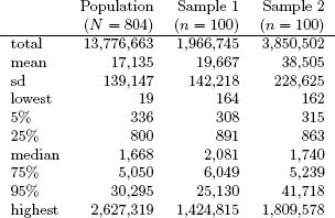
Goal: estimate total population of New York State from samples of 100 municipalities
- Assume normal distribution.
⇒ 95% confidence bounds [2.0×10⁶, 37.0×10⁶]. - Lognormal distribution more appropriate
⇒ [5.4×10⁶, 9.9×10⁶].
This is good right ? -
Posterior predictive check
Test statistic: \(T(y_{\text{obs}}) = \sum_{i=1}^n y_{\text{obs},i}\)
Produce \(S\) independent replicate datasets, and see where the test statistic fits.- Draw \(μ,σ^2\) from posterior, produce \(y_{\text{obs}}^{\text{rep}}\) \,.
- Compute \(T(y_{\text{obs}}^{\text{rep}})\) for each.
sample min
- Extend model to “power transformed normal family”.
Posterior predictive check now gives 15 out of 100 samples with larger sample total.
95% confidence bounds: [5.8×10⁶, 31.8×10⁶] - New problem: this doesn't work on sample 2.
Predicts median of 57×10⁷.
How can the inferences for the population total in sample 2 be so much less realistic with a better-fitting model than with a worse-fitting model ?
The problem with the inferences in this example is not an inability of the models to fit the data, but an inherent inability of the data to distinguish between alternative models.The inference for ytotal is actually critically dependent upon tail behavior beyond the quantile corresponding to the largest observed \(y_{\text{obs}, i}\).
We were warned, in fact, by the specific values of the posterior simulations for the sample total from sample 2, where 10 of the 100 simulations for the replicated sample total were larger than 300 million!
The substantive knowledge that is used to criticize the power-transformed normal model can also be used to improve the model. Suppose we know that no single municipality has population greater than 5 × 10⁶. To include this information in the model, we simply draw posterior simulations in the same way as before but truncate municipality sizes to lie below that upper bound.
For the purpose of model evaluation, we can think of the inferential step of Bayesian data analysis as a sophisticated way to explore all the implications of a proposed model, in such a way that these implications can be compared with observed data and other knowledge not included in the model.
We should also know the limitations of automatic Bayesian inference. Even a model that fits observed data well can yield poor inferences about some quantities of interest. It is surprising and instructive to see the pitfalls that can arise when models are not subjected to model checks.
Bayesian approach gives us more flexible means to incorporate substantive knowledge
Selected Gelman quotes
- “In statistics it’s enough for our results to be cool. In psychology they’re supposed to be correct. In economics they’re supposed to be correct and consistent with your ideology.”
- “Sometimes classical statistics gives up. Bayes never gives up . . . so we’re under more responsibility to check our models.”
- “There are two types of models. Good models, if they don’t fit, you get a large standard error. Bad models, if the model doesn’t fit, it goes . . . [deep voice] No problem. I have a great compromise for you.’ ”
- “In cage 1, they all die, and then in cage 2 they all hear about it, and they’re like, ‘Don’t eat that shit, man.’” (violation of independence assumption in rats data)
- “If I’m doing an experiment to save the world, I better use my prior.”
- (on priors) “They don’t have to be weakly informative. They can just be shitty.”
- “Inference is normal science. Model-checking is revolutionary science.”
- (Someone asks how to compare models. Gelman writes in giant letters: OUT OF SAMPLE PREDICTION ERROR.) “So there’s that.”
- “A Bayesian version will usually make things better.”