Belief Elicitation
|
Alistair Wilson Caltech Experimental Summer School June 2025 |


David
Danz
Pittsburgh

Lise
Vesterlund
Pittsburgh
Beliefs
- Beliefs and expectations are an integral part to our models of choice
- And as such we might want to measure and test them
- See Manski (2004)
- But beliefs are typically not revealed by decisions
- As our approach in economics is mostly through choice, if we want to have incentivized beliefs, then we need elicitation techniques that can reveal them without bias
Beliefs
Different types of beliefs we might care about:
- Subjective confidence over a task/ranking
- Expected wage on getting a degree
- Expected bid by another player in an auction
- Expected value of a lottery
- Posterior probability after receiving a noisy signal
Beliefs: Environment
- Experiment asks agents to make a choice \(x\) over a set \(X\)
- Set of states of the world \(\Omega\), representing some uncertainty
- Agents belief over \(\omega\in\Omega\) represented by \(\theta_i\)
- Initially let's be vague over the belief \(\theta_i\) where examples could be
- Probability of a high-value realization, \(p_\text{High}\)
- Probability distribution over \(\omega\)
- A summary statistic for a distribution, etc.
Beliefs: Environment
- Preference model in an experiment represented by \[\mathbb{E}_\omega u\left(\pi(x,\omega);\theta\right)\]
- We control the incentives \(\pi\) and choice set \(X\) experimentally
- We observe the agent's choice \(x_i\) from the given set
- But separating between two competing models of choice \(u\) or \(\tilde{u}\) might require the analyst to have some measure of \(\theta\)
- Similarly, where we can measure \(\theta\) it can help us understand mechanisms as we posit new models \(u^\star\)
Beliefs: Example 1
- Niederle & Vesterlund (2007) find that women enter a tournament at a lower rate than men, preferring a piece-rate incentive
- Is this aversion to competition driven by:
- A direct preference for not engaging in competition
- Different risk aversion (curvature over the utility function)
- Differences in confidence (probability of winning the auction)
- To understand how confidence affects the decisions, we need to measure it to separate between the competing motives
- While the measured belief is also used as a LHS variable, the main use here is as a RHS control
Beliefs: Example 1
Measured belief here is used in a regression:
Beliefs: Example 2
- In models of belief formation/updating the agent starts from an initial prior distribution, where the task is to update in response to new information
- The standard model here is Bayesian
- Do decision makers approximately follow this, or do they show systematic biases?
- Experiments will vary the prior and information structure
- Need machinery to elicit the posterior beliefs at each point
- Can compare the measured response to the Bayesian rule
- The beliefs here are collected as a LHS variable to see how they are driven by priors, information and behavioral biases, though sometimes they become RHS variables too (the interim priors)
See Benjamin (2019) for a detailed literature review
Beliefs: Example 2
Measured belief used in a Grether regression:
Eliciting Beliefs
- One option here is simply to ask them to tell you \(\theta\)
- This is typically the simplest elicitation, and where this is the standard in most non-experimental economics applied research (Haaland et al 2023)
- Downside to unincentivized beliefs are that you are more likely to get default/less-considered responses
- Unincentivized beliefs are thought to be less effective when:
- There are concerns about ego or partisanship
- What are the chances you have the top score in the IQ test?
- The belief requires some calculation
- Given a red ball was drawn, what is the chance Urn A was selected?
- Understanding the belief construct involves substantial comprehension
- Please specify your subjective probability distribution over the state?
- There are concerns about ego or partisanship
Should we even pay!?
- Overall the lab evidence favors incentives
- But probably fair to consider this not unambiguous
- There is evidence that paying helps reduce biases in Bayesian updating problems (Grether, 1980; Burford & Wilkening 2022)
- Incentieves make beliefs more precise in subjective tasks (Gächter & Renner 2010; Wang, 2012)
- Incentives reduce the frequency of default answers (e.g. 50%)
- Incentives reduce noise (Camerer & Hogarth 1999, Gächter &
Should we even pay!?
- However there is evidence in some studies that:
- Incentives have no effect (Sonnemans and Offerman 2001; Trautmann and van de Kuilen 2015) over flat payment
- Incentives can interact with other decision features:
Eliciting Beliefs
- The other option is provide incentives
- But designing these incentives is not trivial!
- Essentially you have a hidden type \(\theta\in\Theta\) where you need to construct a mechanism \(\phi:\Theta\rightarrow X\) that offers a different incentive \(\phi(\theta)\) for each type
- Our mechanism must satisfy an incentive compatibility condition for all types \(\theta\). That is for all potential alternate reports \(\theta^\prime\in \Theta\setminus\left\{\theta\right\}\) we require:\[u\left(\phi(\theta ),\theta\right)> u\left(\phi(\theta^\prime),\theta\right) \\ u(\textit{Truth})\ \ > u(\textit{Distort})\ \ \ \]
- Note that we use the direct mechanism without loss of generality, but experimentally, in most cases it's better to restrict attention to the direct mechanism
Eliciting Beliefs
- Our mechanism must satisfy an incentive compatibility condition for all types \(\theta\). That is for all potential alternate reports \(\theta^\prime\in \Theta\setminus\left\{\theta\right\}\) we require:\[u\left(\phi(\theta ),\theta\right)> u\left(\phi(\theta^\prime),\theta\right) \\ u(\text{Truth})\ \ > u(\text{Distort})\ \ \ \]
- Non-incentive-compatible mechanisms perform poorly (see Palfrey and Wang 2009)
The main challenge in belief elicitation is that we need to be correct in our theoretical assumptions over the mechanism, at the individual level
- As we're often using beliefs in regressions as LHS and RHS variables we can't just trust in some averaging process in the noise!
Eliciting Beliefs
- Our mechanism must satisfy an incentive compatibility condition for all types \(\theta\). That is for all potential alternate reports \(\theta^\prime\in \Theta\setminus\left\{\theta\right\}\) we require:\[u\left(\phi(\theta ),\theta\right)> u\left(\phi(\theta^\prime),\theta\right) \\ u(\text{Truth})\ \ > u(\text{Distort})\ \ \ \]
-
Experiments are key here to actually checking that theoretical compatible. mechanisms are actually working as theorized!
- By inducing the belief/type, we can check what they report within the mechanism!
Scoring rules, Multiple pricelists & BDMs
Scoring Rules
- For each response \(q\) and state realization \(\omega\) there is an assigned score \(s_\omega(q)\) in the reward medium
- An incentive-compatible scoring rule is strictly proper when the unique best response is to submit the true belief \(q^\star(\theta)=\theta\)
Let's look at eliciting a probability of an event \(E\) (a binary outcome)
- State realization is either the event happens or it does not
- Because we're tied to randomness, payments are naturally lotteries
- True belief is a probability \(\theta\) over the event
- So the scoring rule yields a different lottery depending on the report \(q\): \[\mathcal{L}_\theta(q)=\theta \cdot s_E(q) \oplus (1-\theta)\cdot s_{E^c}(q)\]
Scoring Rules
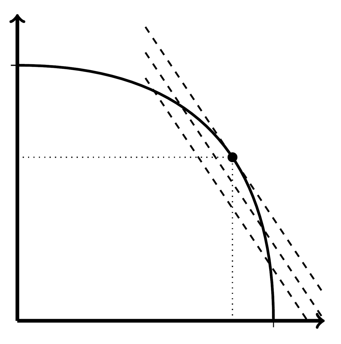
- Supposing that decision maker's preferences over \(\mathcal{L}_\theta(q)\) are linear (with a slope governed by \(\theta\)) over the score
- Scoring rule is bundle of offered payoffs, needs to be strictly convex for proper scoring rule
- One obvious candidate here is to use quadratic loss:
- \(s_E(q)=1-(1-q)^2\)
- \(s_{E^c}(q)=1-(0-q)^2\)
Score on \(E\)
Score on \(E^c\)
\(s_E(\theta)\)
\(s_{E^c}(\theta)\)
\(U(\mathcal{L}_\theta(q)|\theta)\)
\(U(\mathcal{L}_\theta(\theta)|\theta)\)
Scoring Rules
- Quadratic-loss (in reward medium) scoring rule proportional to:
- \(s_E(q)=1-(1-q)^2\)
- \(s_{E^c}(q)=1-(0-q)^2\)
- With linear treatment of the event probability this leads to the outcome: \[1 -\theta\cdot(1-q)^2-(1-\theta)\cdot q^2 \] which is uniquely maximized with \(q^\star(\theta)=\theta\)
- When would we have linear preferences like this!?
- Risk-neutral expected prize (money is treated linearly)
- EU decision maker (reward medium is a probability of winning a prize)
Scoring Rules
| Rule | ||
|---|---|---|
| Quadratic | ||
| Spherical | ||
| Logarithmic |
\(s_E(q)\)
\(s_{E^c}(q)\)
\(1-(1-q)^2\)
\(1-(0-q)^2\)
\(\frac{q}{\sqrt{q^2+(1-q)^2}}\)
\(\frac{1-q}{\sqrt{q^2+(1-q)^2}}\)
\(\ln(q)\)
\(\ln(1-q)\)
- For binarized rule, quadratic has the strongest average incentives
- Spherical rules have stronger incentives closer to the midpoint
- Logarithmic rules have stronger incentives closer to the extremes, but note that they cannot be binarized
Multiple Price Lists
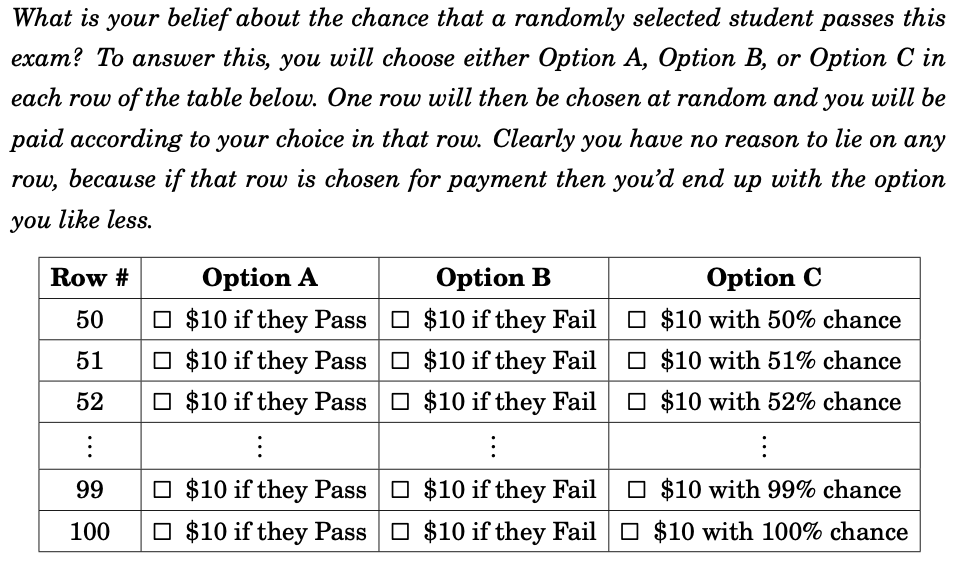
- An alternative to scoring rules is to use a price list, where we ask the participant to make a choice between a subjective and an objective act
- Each comparison in the list asks about an ordinal response:
| Row # | Option A | Option B |
|---|---|---|
| 0 | $X on E | $X with 0% chance |
| 1 | $X on E | $X with 1% chance |
| 2 | $X on E | $X with 2% chance |
| 3 | $X on E | $X with 3% chance |
| 99 | $X on E | $X with 99% chance |
| 100 | $X on E | $X with 100% chance |
\(\vdots\)
\(\vdots\)
\(\vdots\)
Multiple Price Lists
| Row # | Option A | Option B |
|---|---|---|
| 0 | $X on E | $X with 0% chance |
| 1 | $X on E | $X with 1% chance |
| 2 | $X on E | $X with 2% chance |
| 3 | $X on E | $X with 3% chance |
| 99 | $X on E | $X with 99% chance |
| 100 | $X on E | $X with 100% chance |
\(\vdots\)
\(\vdots\)
\(\vdots\)
- Choose one of the 101 rows, and pay the participant based on their answer
- Dominant to choose option B whenever the objective chance exceeds your subjective belief on \(E\)
Multiple Price Lists
| Row # | Option A | Option B |
|---|---|---|
| 0 | $X on E | $X with 0% chance |
| 1 | $X on E | $X with 10% chance |
| 2 | $X on E | $X with 20% chance |
| 3 | $X on E | $X with 30% chance |
| 99 | $X on E | $X with 90% chance |
| 100 | $X on E | $X with 100% chance |
\(\vdots\)
\(\vdots\)
\(\vdots\)
- Choose one of the 11 rows, and pay the participant based on their answer
- Dominant to choose option B whenever the objective chance exceeds your subjective belief on \(E\)
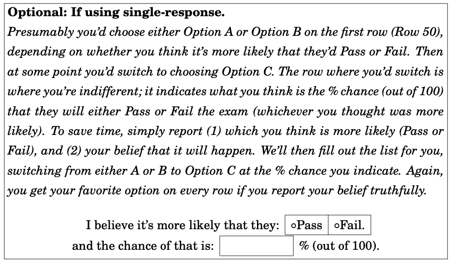
Single-response BDM mechanism
- Can create a mechanism that acts like the MPL, but where we ask for the switch point
- Randomly draw some \(r\in[0,1]\) (typically a uniform draw)
- Have the agent choose the threshold \(q\in[0,1]\) where they would switch from Option A to Option B
-
After choosing \(q\) they are told the realization of \(r\) and receive:
- ( The \(\$X\) prize on \(E\) ) whenever \(r\leq q\)
- (The \(\$X\) prize with prob. \(r\)) whenever \(r>q\)
- Similar to the MPL, under weaker restrictions on the preferences, we have that it is optimal to report \(q^\star(\theta)=\theta\) the subjective probability placed on \(E\)
Single-response BDM mechanism
- The marginal incentives in the BDM are half the size of the BSR: you give more of the incentive away for free!
- Unclear that participants recognize this though
How do these mechanisms actually function?
Quadratic Scoring Rule (QSR)
- Quadratic scoring was the initial main workhorse for belief elicitation
- Here the reward medium is dollars, so the belief paid a reward of \[\$(A-c\cdot(\omega-q)^2)\]
- For binary events the QSR lead to the lottery reward: \[\phi(q;\theta)=\theta\cdot \$(A-c\cdot(1-q)^2) \oplus (1-\theta)\cdot \$(A - c\cdot q^2)\]
- The mechanism is only incentive compatible for risk neutral EU decision makers
- Authors/reviewers worried that risk aversion would push the agent towards the center where they got a certain payment
- (There's an inherent tension in a field trying to understand behavioral decision making enforcing very strong theoretical assumptions in their secondary measurement techniques!)
Quadratic Scoring Rule
Fraction not reporting induced prior
Expected deviation by induced prior
Quadratic Scoring Rule (QSR)
- Two main proposals arose:
- Modify the measured beliefs to correct for risk aversion
- Find scoring rules that worked under less restrictive assumptions
- The first approach is examined in Offerman et al.
- Calibrate the elicited beliefs through an initial array of objective elicitations
- Estimate a structural model of risk to correct the subjective beliefs (treating the QSR like an indirect mechanism at subject level)
- The literature instead followed the second approach:
- Applied a common trick in experimental methods to avoid risk aversion critiques: pay with probabilities
Binarized Scoring Rule (BSR)
-
Hossain and Okui (2013) examine the properties of the binarized scoring rule:
- Uses Roth & Malouf (1979) idea of paying in probabilities
- Theoretically works under a slight relaxation of EU because of restriction to a binary domain
- Stochastic dominance and reduction of compound lotteries
- Paper examines a clear test of the QSR vs BSR
- Find reduced distortions in eliciting a proportion (here known proportion of balls in an urn)
BSR vs QSR horserace
Reduced distortions, and no differential effect across risk aversion (here using a meta-study dataset from Danz et al. 2024)
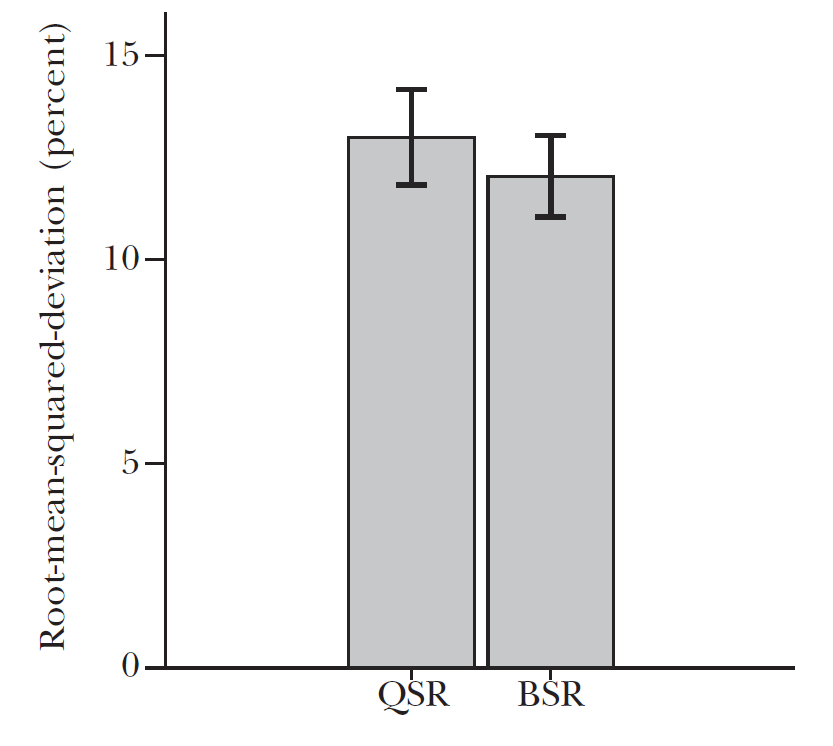
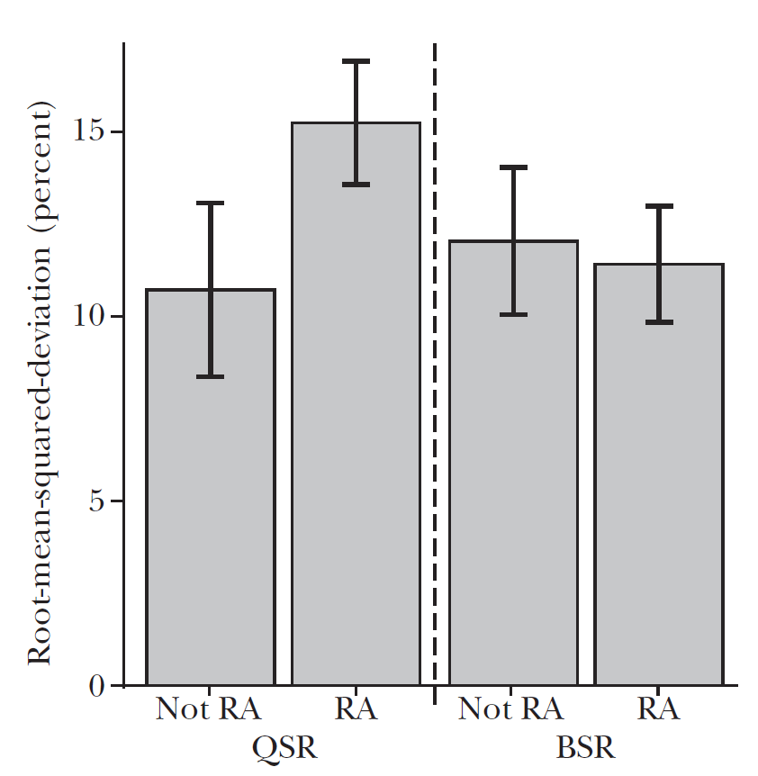
BSR vs QSR horserace
- Given the relative improvement in performance, and the easier to defend theoretical assumptions, BSR became the most popular elicitation
Deeper Examination of the BSR
- Danz et al (2022) offers a more direct test of the mechanism's incentive compatibility
- Fix the mechanism, but focus on design-by-subtraction to examine the effects of the incentives
- Bayesian updating environment:
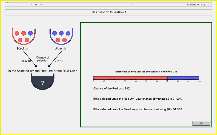
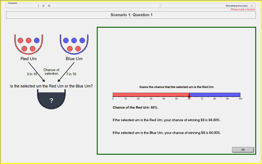
Danz et al. (2022)
Task
Each belief scenario consists of three seperate elicitations.

- Guess 1: Prior
- Guess 2: Posterior
- Guess 3: Posterior


Danz et al. (2022)
- 5 treatments
- Treatment variation: Information on incentives
- Holding constant across treatments
- Incentives
- Experimental procedures
- All scenarios and random draws matched
- 60 participants per treatment (3x20)
- Written instructions read out loud, slide summary
- 10 scenarios with random draws (30 elicitations total)
- Payment
- $8 show up
- $8 prize with one guess paid from two scenarios
- One participant per session paid for end-of-experiment elicitations
Baseline: Information Treatment
| Property | Information |
|---|---|
| Dominant Strategy | |
| Payoff Description | |
| Payoff Slider | |
| Feedback |
✅
✅
✅
✅
✅
✅
✅
✅
Instructions:
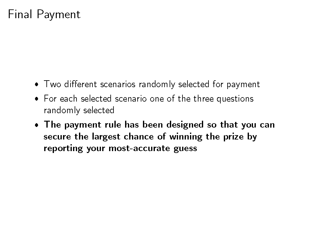
The payment rule is designed so that you can secure the largest chance of winning the prize by reporting your most-accurate guess.
Slide summarizing instructions:
(literally the last thing they see
before they begin making decisions)
Baseline: Information Treatment
- Randomly draw two uniform numbers between 0-100
- If the selected urn is the Red urn: You will win the $8 prize if Your Guess is greater than or equal to either of the two Computer Numbers.
- If the selected urn is the Blue urn: You will win the $8 prize if Your Guess is less than either of the two Computer Numbers.
- Yields the BSR lottery probabilities (Wilson & Vespa 2018)
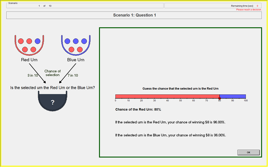
Payoff Slider
Feedback
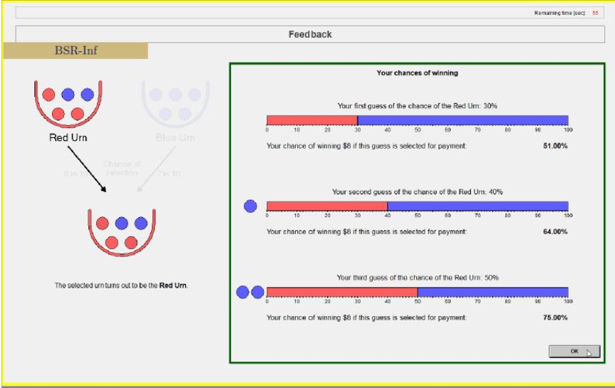
At the end of each round:
- Realized urn
- Earned probability on each elicitation
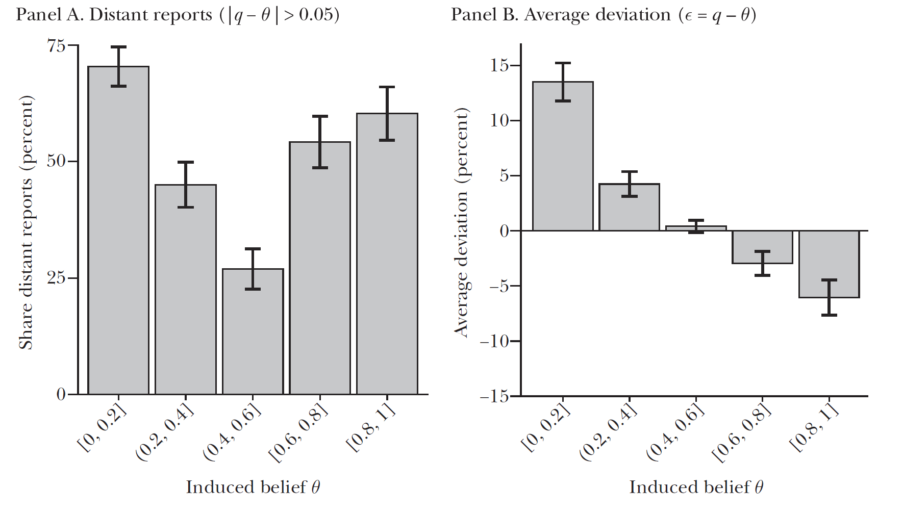
Results in Information Baseline
Only 15 percent of participants consistently report induced prior
Results in Information Baseline
Only 15 percent of participants consistently report induced prior
BSR Payoffs
- Reporting a belief toward center
- large increase in chance of winning on unlikely event
- smaller decrease in chance of winning on likely event
84% chance
83% chance
- Cheap false reports:
- 10% pt deviation from truth reduces chance of winning by 1% pt
| Stated Belief on Red | Chance to Win if Red | Chance to Win if Blue |
|---|---|---|
| 1 | 100% | 0% |
| 0.9 | 99% | 19% |
| 0.8 | 96% | 36% |
| 0.7 | 91% | 51% |
| 0.6 | 84% | 64% |
| 0.5 | 75% | 75% |
BSR Payoffs
| Reporting rule | Earnings |
|---|---|
| Truthful | $6.27 |
| Middle | $6.00 |
| Random | $5.33 |
| Minimizing | $2.88 |
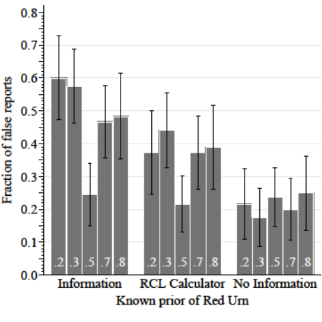
False Reports vary by True Prior
- False reports more likely on non-centered than centered priors
- Deviations more likely toward center than near extreme (reports pull-to-center)
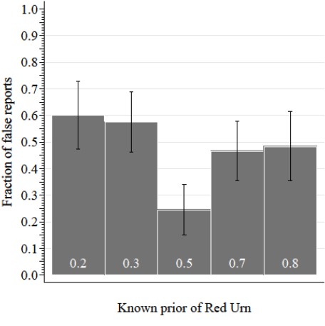
False Reports tended to the Center
- Example of the reports with a prior of 0.3

Near-extreme
Center
Distant-extreme
Proportion of non-centered reports in each bin:
- Confusion
-
Incentives
-
Failure to reduce compound lottery
-
flatness
-
asymmetry
-
-
Vary information on incentives:
-
RCL-calculator : Aid reduction of compound lottery
-
No-Information: Eliminate quantitative information on incentives
-
Cause of false BSR reports?
Treatment variation
✅
✅
✅
✅
❌
✅
✅
✅
✅
❌
- RCL adds information on the incentives
- No Information subtracts information
| Property | Information | RCL | No-Information |
|---|---|---|---|
| Dominant Strategy | | ||
| Payoff Description | | ||
| Payoff Slider | | ||
| Feedback | | ||
| RCL calculator | |
✅
❌
❌
❌
❌
✅
✅
✅
✅
✅
Treatment variation
| Treatment | Source of false reports |
|---|---|
| Information | confusion, BSR incentives, failed RCL |
| RCL | confusion, BSR incentives |
| No Information | confusion |
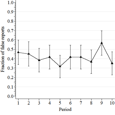
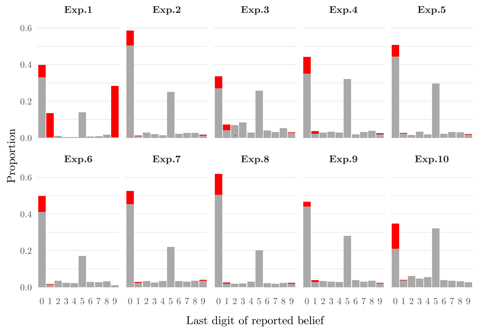
False Reports by Round
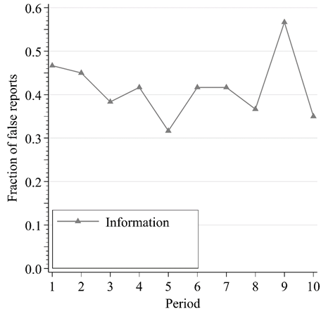
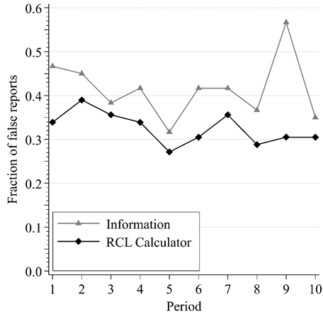
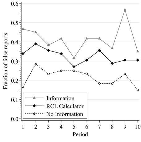
Truthful reporting greatest w/o incentive information
False Reports by Prior
Movement of false reports
Near-extreme
Center
Distant-extreme
Proportion of non-centered reports in each bin:
Inf:
RCL:
NoInf:
Does this matter at all for inference?
To understand the effects on inference we use a simple model of the center-bias distortions
Observed belief is:
Regression model where X is a binary treatment indicator:
What happens when distorted beliefs are used?
Does this matter at all for inference?
Observed belief is:
Left-hand-side effect is clear:
- Mismeasurement of q leads to an attenuation of the estimated treatment effect
Does this matter at all for inference?
Observed belief is:
Right-hand-side treatment effect will depend on unknowns:
Test Inferential effect with a replication
We return to the Niederle & Vesterlund study:
- Perform sums for a piece rate
- Perform sums in tournament
- Choose the preferred incentive
-
Elicit subjective belief
- (here using BSR)
Run this study twice:
- NV-Information: Information
- NV-No-Information : NoInformation
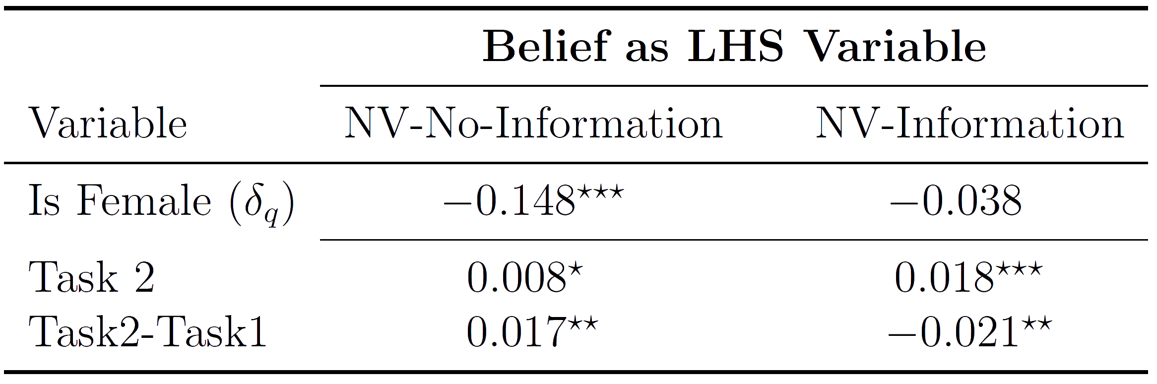
Test Inferential effect with a replication
LHS: Confidence difference between men and women:
RHS: Competition difference for men and women after controlling for confidence:
Information predicted to attenuate gender confidence difference
Information predicted to make the gender-gap in tournament-entry larger (after controlling for confidence
Test Inferential effect with a replication
Original finding is that:
- Women are less confident over their performance than men
- Prediction from model for NV-Information is that gender gap will move towards zero.
Test Inferential effect with a replication
- Original finding is that:
- Beliefs explain a significant proportion of the gender gap
- Prediction from model for NV-Information is that gender gap in competition is more negative:
- (gender gap in confidence)
- (Belief effect on entry)
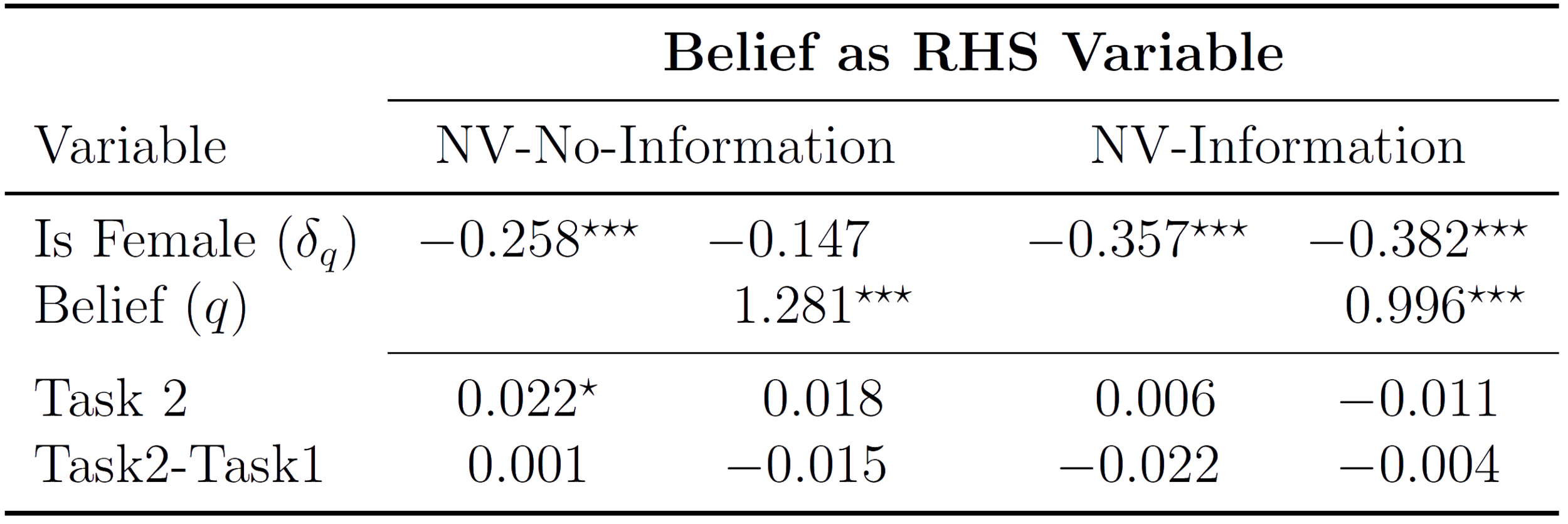
Replication conclusions
- NV-Information distorts beliefs to center, relative to NV-No-Information
- This difference in the beliefs affects final inference:
- As a LHS variable it attenuates the treatment effect (here a gender gap over beliefs)
- As a RHS variable it widens the measured gender gap over competition after controlling for beliefs
- So, simply by providing the participants with information on the elicitation incentives, that we can qualitatively distort the subsequent inference
Multiple Pricelists
- The Healy and Leo chapter on belief elicitation is very positive on price lists
- PROS:
- They are incentive compatible under very weak assumptions on preferences
- CONS:
- They are slow to fill out
- They take up a lot of screen real-estate
- SUPER CON:
- Some of your participants will misunderstand and have multiple switch points
MPLs and BDMs
-
Holt & Smith (2016) find evidence favoring a modified (crossover) MPL over both the QSR and the BDM
- Closer to induced prior and bayesian posteriors
- Healy & Kagel (presentation) find similar performance between a BDM and the BSR
- PJ's preferred implementation is:
- Enforce a single switch point
- (I'm not sure I fully understood their better to have measurement error than having to make parametric assumption! argument)
- Use a textbox entry rather than slider, have the price list in it's own scrollable box; after entering the belief, the list is auto-filled
- Enforce a single switch point
Tenary Elicitation
- Healy and Leo have a more-compact MPL implementation for eliciting probabilities:
Tenary Elicitation
- Healy and Leo have a more-compact MPL implementation for eliciting probabilities:
Pricelists, BDMS and Tenary Methods
- Healy and Leo do have data, though I've only seen it in a presentation thus far
- Suggests pricelists and tenary elicitation do about as well BQSR without information on the incentives
Alternate elicitations: the Mode
- It's often easier to incentive the mode if you have multiple realizations or an outcome with an intensity
- Can ask participants for a particular realization
- pay them if they are correct
- or within a specified interval of the realization
Alternate elicitations: the Median
- We can alter the BSR/QSR scoring rules to elicit the median (or other quantiles of the distribution) by switching out the quadratic loss for linear loss:
- Parallels here with econometrics:
- OLS (minimizing quadratic loss) estimates the expectation
- LAD (minimizing the absolute deviation) estimates the median
- Can generalize to any quantile same as quantile regression through relative slopes of the loss function either side of realized outcome
- Parallels here with econometrics:
Other Concerns: Mismeasurement
- A number of papers have become concerned with understanding how errors in reported beliefs affect estimates:
- To what extent can measurement error in the prior generate base-rate neglect in Grether belief regressions
- Mobius et al. (2022) try to mitigate this by instrumenting for the prior
- To what extent can measurement error in the prior generate base-rate neglect in Grether belief regressions
- Bland and Rosokha (2024) take this further by considering the effects of rounding errors in a meta-study of updating experiments
Other Concerns: Rounding
Other Concerns: Rounding
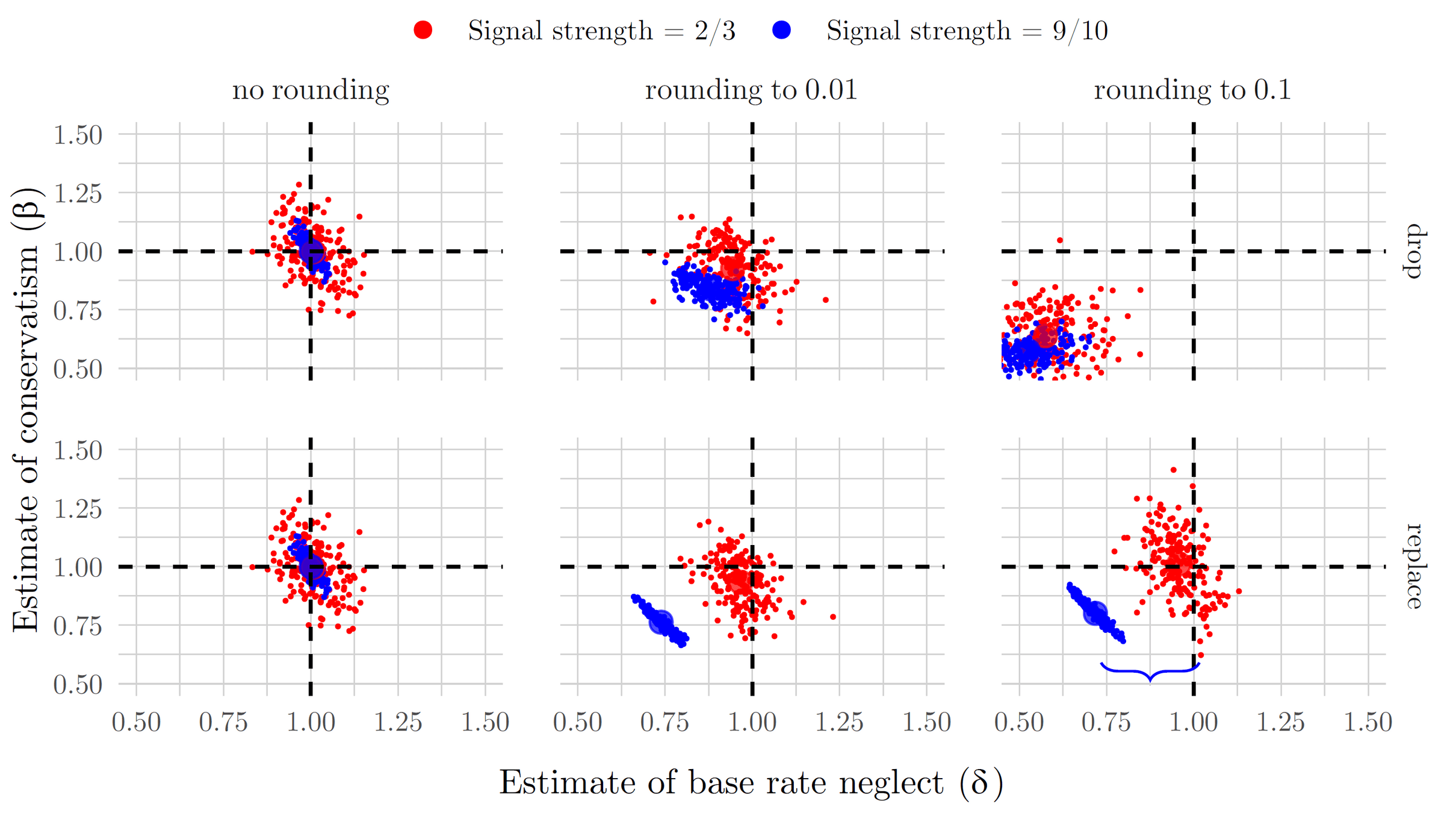
- Grether regressions for Bayesian agents (drop/replace is for boundary decisions)
Other Concerns: Inducing Effort
0
100
20
80
Suppose that forming a clearer belief requires effort
Other Concerns: Inducing Effort
0
100
20
80
Supposing that forming a clearer belief requires some effort
Other Concerns: Inducing Effort
- So now we have two incentive problems!
- We continue to want incentive compatibility of truthful reporting (so no distortions)
- But we also want the incentives to be steep enough so that the marginal benefits of effort exceed the marginal costs!
- Elicitations using a binary event realization are necessarily very flat, so they offer little marginal benefit from effort!
Inducing effort with Elicitations
- Task that mirrors forming a probabilistic belief but that also clearly requires effort to refine it
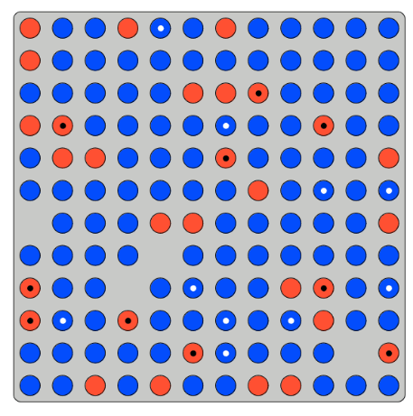
- What is the proportion of blue tokens in this urn?
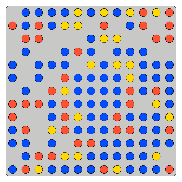
Ans: 56.25%
Working project with Brandon Williams:
Inducing effort with Elicitations
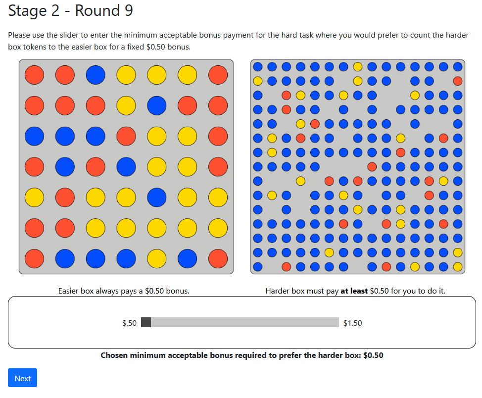
Ten rounds: Elicit cost for an easy task, or a Hard one plus amount \(\$X\)
LHS:
Constant
Difficulty
RHS:
Varying
Difficulty
Always
Pays $.50
If Correct
$X
If Correct
Choose
$X threshold
Inducing effort with Elicitations
\(\text{OLS }(\text{Effort})\)
\(\text{Tobit}(\text{WTA})\)
\(\text{Logit }(\text{Correct})\)

Output

Effort

WTA
Our calibration demonstrate that the task responds to effort, is costly, and in a set of other experiments, we obtain their low-effort guesses
Inducing effort with Elicitations
After 15 second
After 45 second


Inducing Effort with Elicitations
Use four incentives to ask about beliefs in ten different urns:
-
BSR-Desc: $1.50 prize with only qualitative information on the details
- Text description of payoff structure (Vespa & Wilson, 2018)
-
BSR-Inf: as above but with quantitative information
- Full information on the quantitative incentives (Danz et al., 2022)
- BSR-NoInf: only know there is a $1.50 prize, no other information on the incentives
- A "close enough" modal incentive
- $1.50 if within 1% of true realization; $0.50 if within 5%
- Current use in several papers now (e.g. Ba et al., 2024)
- Pay three of the ten rounds
- \(N=100\) each incentive treatment
Inducing effort with Elicitations

Model:
- Urn is \(\text{Binomial}(\theta,n)\)
- Prior is \(\theta\sim \text{Beta}[1,1]\)
- Posterior after counting \(k\) balls from \(n\) is \(\text{BetaBinomial}[1,1,n,k]\)
Inducing effort with Elicitations

Inducing effort with Elicitations
- "Close enough" outperforms BSR on both accuracy and time spent
- The better incentive effects stemming from a richer outcome space
- Also cheaper for the experimenter, incentive payments to participants reduced by ~50% over BSR
- (With a fixed budget, how much more effort could be induced?)
Inducing effort with Elicitations
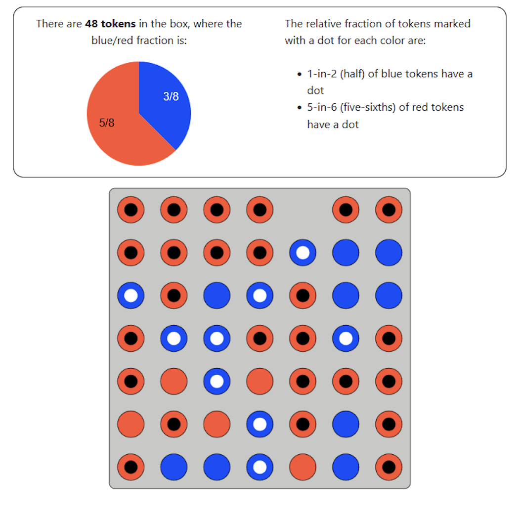
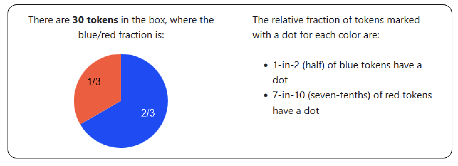
Participants told:
- Number of tokens
- Proportion blue
- Proportion Dots | Blue
- Proportion Dots | Red
Are then asked for the proportion of blue balls given a dot:
- Calculation identical to standard Bayesian updating experiments
- But can also just count...
We then elicit the costs for performing the Bayesian update calculation:
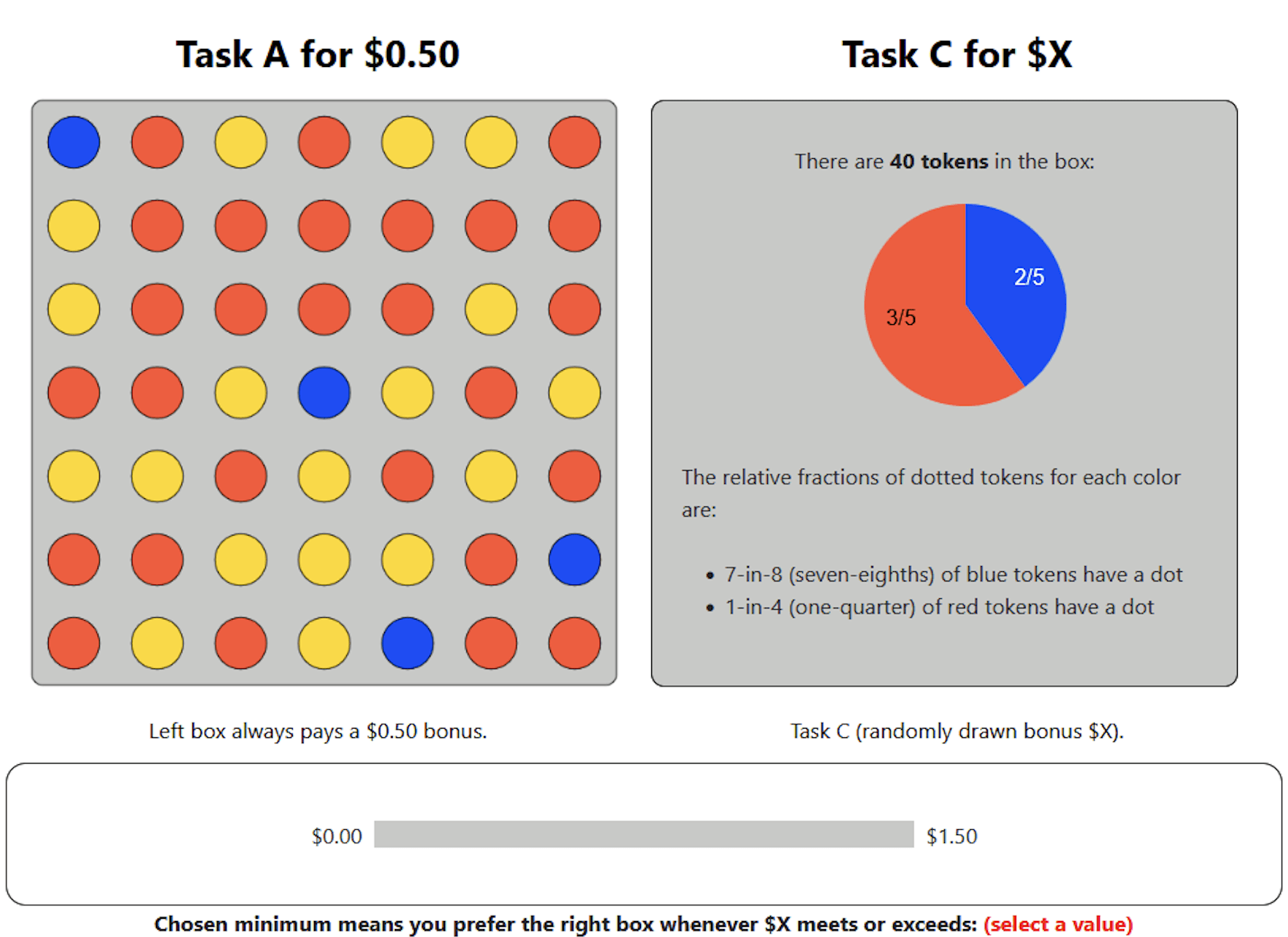
Inducing effort with Elicitations
Calc or Count
Calc only
Proportion of Blue dotted tokens
Inducing effort with Elicitations
Can they perform each task?

Inducing effort with Elicitations
Elicit how much they require to do the task:
Inducing effort with Elicitations
For those who can do the calculation


For those who can't
Avg: $0.82
Avg: $0.99
Inducing effort with Elicitations
- For our Bayesian updating task:
- 50% or Prolific subjects can perform the calculation if given frequentist version
- But the reward needs to be ~$0.55 per problem to offset costs
- So beyond incentivizing truthful reporting, suggests that we also need to more clearly pay for the costs of the calculation
Recommendations from Healy & Leo
- On Incentives
- Use incentives, but don't put them on the decision screen
- Do say that truthtelling is optimal!
-
For beliefs about a number, avoid eliciting the mean consider eliciting the mode (or modal interval) instead
-
For beliefs about a frequency, consider eliciting the probability of a single, randomly chosen outcome
-
Consider coarser elicitations
-
Use a pricelist for probabilities; however, if committed to a scoring rule use the BQSR
Going forward...
- New mechanisms focused on simplicity/clarity
- New evidence on what works
- Better econometric modeling:
- Coarser, more-focused elicitation
- Experimental evidence on mechanisms:
- Behavioral incentive compatibility