Behavioral Incentive Compatibility
David Danz
Lise Vesterlund
Alistair Wilson
Exeter, April 2023
Incentive Compatible Mechanisms
How should we pay?
- Ask
- Ask + Pay
- Ask + Pay + Incentive compatible
Experimental economists are often faced with a choice over how to elicit information
Incentive Compatibility
- For each type there is a different uniquely maximizing choice within the mechanism
- This yields fully separating behavior
- Given this one-to-one correspondence, the analyst can interpret the relevant choice as the type
- Elicitation mechanisms are at the sharp end of mechanism design, using the above correspondence for measurement
- Often as an input into inferential regressions
- Subjective beliefs are a clear example, and are often central for inference
Behavioral Incentive Compatibility
- Need to examine the extent to which the theoretical assumptions holds
- Show that a prominent mechanism with relatively weak theoretic conditions for IC is not behaviorally incentive compatible
- Demonstrate the substantive effects of this failure over: Objective probabilities, Objective posteriors, Subjective beliefs
- Use this to motivate two methodological checks to assess Behavioral Incentive Compatibility
Example of Beliefs in Inference:
Niederle & Vesterlund (QJE 2006)
Main Idea:
Paper examines gender & competition:
- Do women compete less than men?
- Use a clever experimental design to examine tournament entry
- Measure beliefs with a very simple elicitation.
Example of Beliefs in Inference:
Niederle & Vesterlund (QJE 2006)
Use of Beliefs:
Use beliefs in two ways:
- As a left-hand-side variable to examine confidence differences between men and women
- As a right-hand-side variable to assess the degree that confidence differences explain gender differences in competition choices
Evolution of Belief Elicitation
- Niederle & Vesterlund used a very simple (and coarse) elicitation device:
- Modal rank in tournament (paying $1 if correct)
- But the literature has increasingly focused on elicitations of arbitrarily precise probabilities
- Initial IC elicitations assumed risk-neutral EU maximizers: Quadratic Scoring Rule (QSR)
- But risk aversion pushes beliefs to center
- One response to this was to control for risk preferences within the elicitation
- Another was to use an elicitation that is IC for a wider set of preferences
-
Houssain & Okui (2013): the Binarized Scoring Rule
-
Belief elicitation in practice:
-
Incentive compatibly. QSR (Brier, 1950), BSR (Roth and Malouf, 1979; Grether, 1980; Allen, 1987; Hossain and Okui, 2013; Schlag and van der Weele, 2013), BDM (Holt and Smith, 2009; Karni, 2009)
-
Surveys (Manski, 2004; Schotter and Trevino, 2014; Schlag et al., 2015)
-
Distortions and corrections (Offerman et al., 2009, Andersen et al., 2013; Harrison et al., 2013; Armantier and Treich, 2013; Schlag and van der Weele, 2013)
-
Stakes and hedging (Blanco et al., 2010; Coutts, 2019)
-
Does elicitation change behavior? (Croson, 2000; Wilcox and Feltovich, 2000; Rutstrom and Wilcox, 2009; Gächter and Renner, 2010)
Belief elicitation in practice:
- Does incentivization matter? (Offerman and Sonnemans, 2004; Gächter and Renner, 2010; Wang, 2011; Trautmann and van de Kuilen, 2014)
-
Does properness matter? (Nelson and Bessler, 1989; Palfrey and Wang, 2009)
-
Consistency with actions (Cheung and Friedman, 1995; Nyarko and Schotter, 2001; Costa-Gomes and Weizsäcker, 2008; Rey-Biel, 2009; Blanco et al., 2011; Ivanov, 2011; Hyndman et al., 2013; Armantier et al., 2013)
-
Models of belief formation (Fudenberg and Levine, 1998; Camerer and Ho, 1999; Nyarko and Schotter, 2001; Hyndman et al., 2012)
-
Bayesian updating (Holt and Smith, 2009; Benjamin, 2019)
-
Higher-order beliefs (Dufwenberg and Gneezy, 2000; Charness and Dufwenberg, 2006; Manski and Neri, 2013)
Binarized scoring rule (Hossain and Okui, 2013)
- Each reported belief q is linked to state-contingent lottery.
- With a binary outcome:
BSR – Binarized scoring rule
- BSR the state-of-the-art in belief elicitation
- Superior theoretical properties: Incentive compatible for individuals aiming to maximize the chance of winning a prize
- Superior performance: Outperforms the standard (non-binarized) quadratic scoring rule (Hossain and Okui, 2013; Harrison and Phillips, 2014)
- Investment and portfolio choice (Hillenbrand and Schmelzer, 2017; Drerup et al., 2017)
- Coordination (Masiliūnas, 2017)
- Matching markets (Chen and He, 2017; Dargnies et al., 2019)
- Biased information processing (Hossain and Okui, 2019; Erkal et al., 2019)
- Cheap talk (Meloso et al., 2018)
- Risk taking (Ahrens and Bosch-Rosa, 2018)
- Information source choice (Charness, Oprea, and Yuksel, forthcoming)
- Memory and uncertainty ( Enke, Schwerter, and Zimmermann, 2020; Enke and Graeber, 2019)
- Discrimination (Dianat, Echenique, and Yariv, 2018)
- Gender and coordination (Babcock et al., 2017)
- Correlated and motivated beliefs (Oprea and Yuksel, 2020; Cason, Sharma, and Vadovič, 2020)
Task
Each belief scenario consists of three seperate elicitations.

- Guess 1: Prior
- Guess 2: Posterior
- Guess 3: Posterior


Initial Design
- 5 treatments
- Treatment variation: Information on incentives
- Holding constant across treatments
- Incentives
- Experimental procedures
- All scenarios and random draws matched
- 60 participants per treatment (3x20)
- Written instructions read out loud, slide summary
- 10 scenarios with random draws (30 elicitations total)
- Payment
- $8 show up
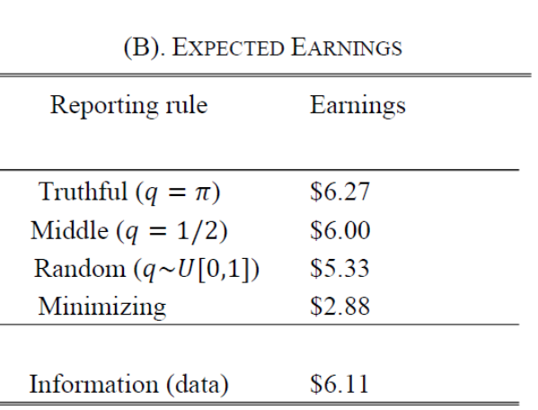
- $8 prize with one guess paid from two scenarios
- One participant per session paid for end-of-experiment elicitations
Baseline: Information Treatment
| Property | Information |
|---|---|
| Dominant Strategy | |
| Payoff Description | |
| Payoff Slider | |
| Feedback |
✅
✅
✅
✅
✅
✅
✅
✅
Dominant Strategy
Instructions:
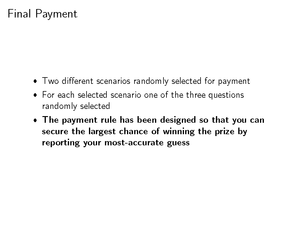
The payment rule is designed so that you can secure the largest chance of winning the prize by reporting your most-accurate guess.
Slide summarizing instructions:
(literally the last thing they see
before they begin making decisions)
Payoff Description
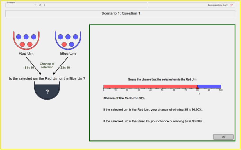
- Randomly draw two uniform numbers between 0-100
- If the selected urn is the Red urn: You will win the $8 prize if Your Guess is greater than or equal to either of the two Computer Numbers.
- If the selected urn is the Blue urn: You will win the $8 prize if Your Guess is less than either of the two Computer Numbers.
- Yields the BSR lottery probabilities (Wilson & Vespa 2018)
Payoff Slider
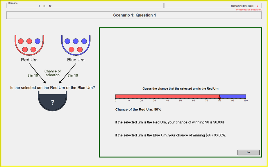
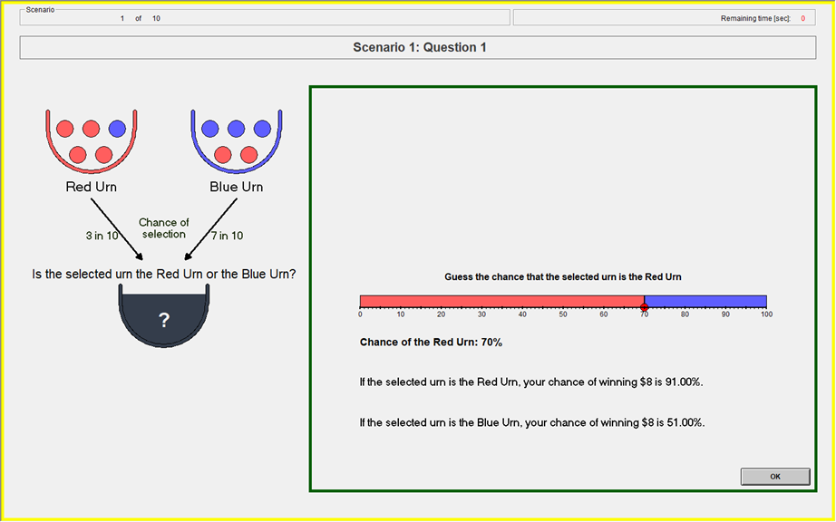
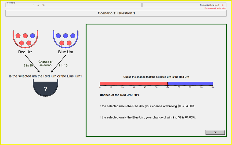
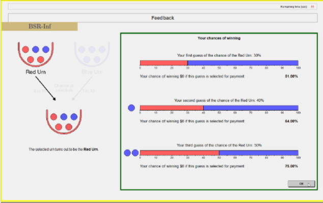
Feedback
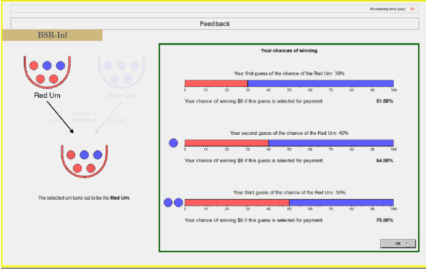
At the end of each round:
- Realized urn
- Earned probability on each elicitation
Results
-
Prior (Guess 1)
-
Posteriors (Guesses 2&3)
Guess 1: Prior Elicitation
Should report induced prior if incentivized to tell truth
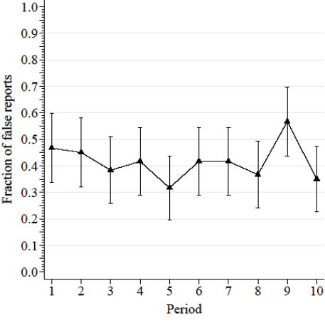
Only 15 percent of participants consistently report given prior
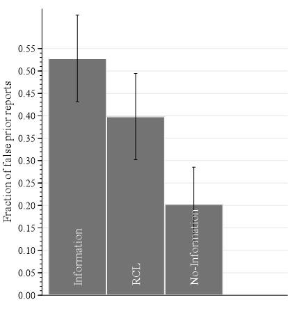
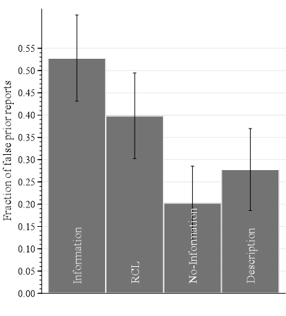
Information: False priors report
What Drives False Reports?
-
Confusion (inability/unwillingness to report given prior)
-
Incentives:
-
Failure to reduce compound lottery (RCL)
-
Payoff structure
-
BSR Payoffs
- Reporting a belief toward center
- large increase in chance of winning on unlikely event
- smaller decrease in chance of winning on likely event
84% chance
83% chance
- Cheap false reports:
- 10% pt deviation from truth reduces chance of winning by 1% pt
| Stated Belief on Red | Chance to Win if Red | Chance to Win if Blue |
|---|---|---|
| 1 | 100% | 0% |
| 0.9 | 99% | 19% |
| 0.8 | 96% | 36% |
| 0.7 | 91% | 51% |
| 0.6 | 84% | 64% |
| 0.5 | 75% | 75% |
What Drives False Reports?
-
Confusion (inability/unwillingness to report given prior)
-
Incentives:
-
Failure to reduce compound lottery (RCL)
-
Payoff structure (asymmetric and flat incentives)
-
Evidence that Incentives drive False Reports
- False reports more likely on non-centered than centered priors
- Deviations more likely toward center than near extreme (reports pull-to-center)
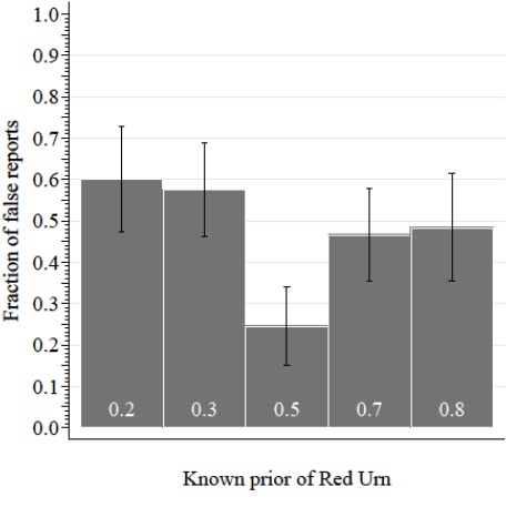


Elicited Priors at 0.3
Near-extreme
Center
Distant-extreme
False-report movements
Proportion of non-centered reports in each bin:
Evidence of incentives distorting reports
- False reports more likely on non-centered than centered priors
- Pull-to-center: Deviations more likely toward center than near extreme
- Survey responses discuss a hedging motive
- Confusion
-
Incentives
-
Failure to reduce compound lottery
-
flatness
-
asymmetry
-
-
Vary information on incentives:
-
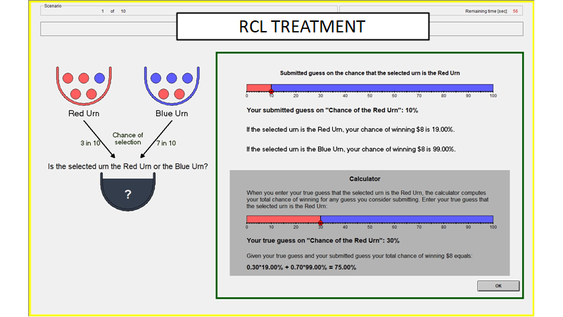
RCL-calculator : Aid reduction of compound lottery
-
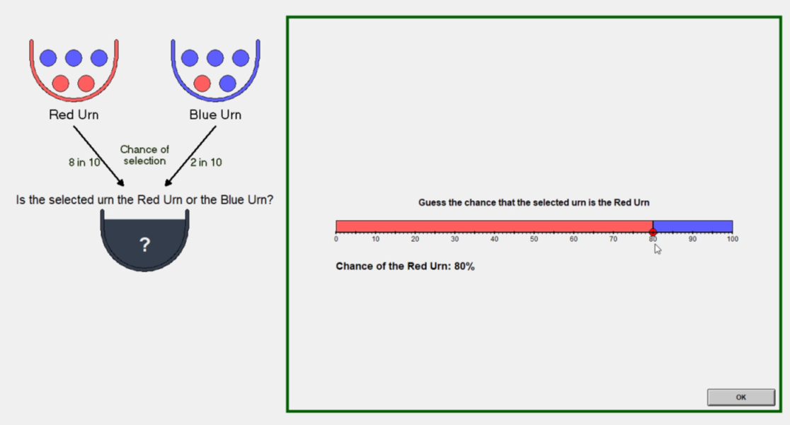
No-Information: Eliminate quantitative information on incentives
-
Cause of false BSR reports?
✅
✅
✅
✅
❌
✅
✅
✅
✅
❌
Treatments:
- RCL adds information on the incentives
- No Information subtracts information
| Property | Information | RCL | No-Information |
|---|---|---|---|
| Dominant Strategy | | ||
| Payoff Description | | ||
| Payoff Slider | | ||
| Feedback | | ||
| RCL calculator | |
✅
❌
❌
❌
❌
✅
✅
✅
✅
✅
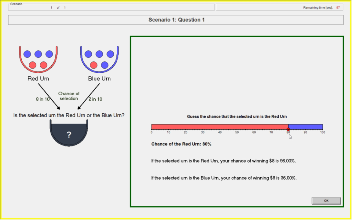
Information treatment
RCL Treatment
No Information treatment
What drives BSR false reports?
| Treatment | Source |
|---|---|
| Information | confusion, BSR incentives, failed RCL |
| RCL | confusion, BSR incentives |
| No Information | confusion |
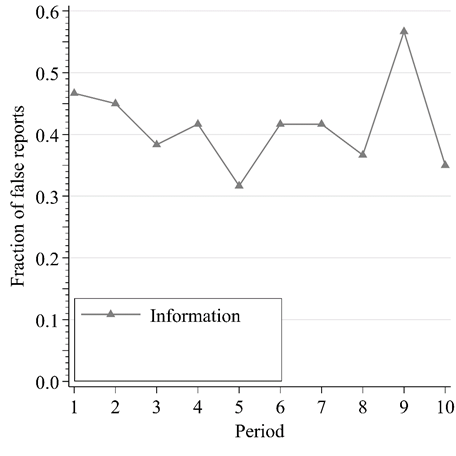
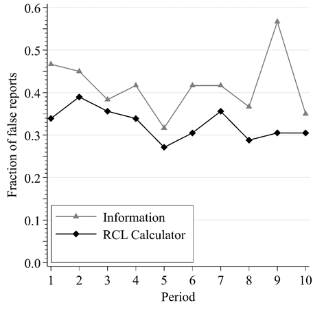
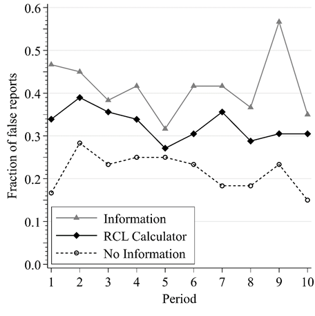
False Reports by Round
Truthful reporting greatest w/o incentive information
False reports by Prior
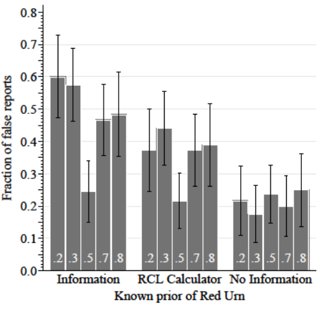
Near-extreme
Center
Distant-extreme
Proportion of non-centered reports in each bin:
Inf:
RCL:
NoInf:
Distribution of false reports
By prior location:
Confusion
BSR Incentives
Compounding
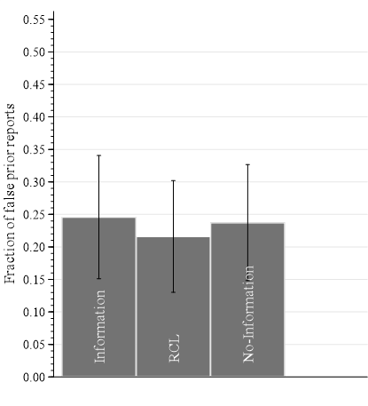
False reports
Centered Prior
BSR Incentives
- Information on BSR incentives increases false reports (by 150%) (between-subject)
- Test effect of information within subject
- Feedback Treatment
- No-Info + scenario feedback with gradual information on incentives
- Feedback Treatment
| Property | Inf | RCL | No-Inf | Feedback |
|---|---|---|---|---|
| Dominant Strategy | ✅ | ✅ | ✅ | ✅ |
| Payoff Description | ✅ | ✅ | ❌ | ❌ |
| Payoff Slider | ✅ | ✅ | ❌ | ❌ |
| Feedback | ✅ | ✅ | ❌ | ✅ |
| RCL calculator | ❌ | ✅ | ❌ | ❌ |
Feedback Treatment
Feedback screen
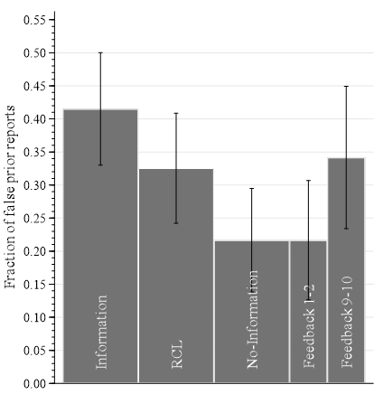
False prior reports
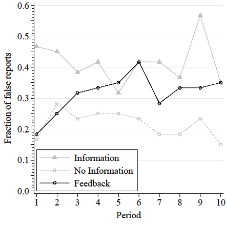
- Starts out at No Information level
- Ends up at Information level
- Information on incentives distorts truthful reporting within subject
False Reports of Prior
Summary so far...
-
Information on incentives increases false reports
-
Between subject: Information vs. No-Information
-
Within subject: Feedback
-
-
What is ‘enough’ information to maintain truth telling?
-
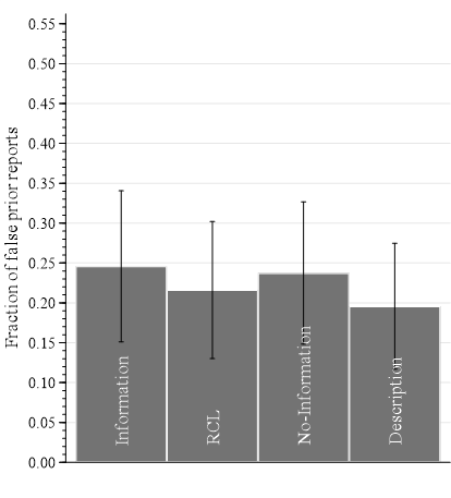
Description Treatment
-
| Property | Inf | RCL | No-Inf | Feedback | Description |
|---|---|---|---|---|---|
| Dominant Strategy | ✅ | ✅ | ✅ | ✅ | ✅ |
| Payoff Description | ✅ | ✅ | ❌ | ❌ | ✅ |
| Payoff Slider | ✅ | ✅ | ❌ | ❌ | ❌ |
| Feedback | ✅ | ✅ | ❌ | ✅ | ❌ |
| RCL calculator | ❌ | ✅ | ❌ | ❌ | ❌ |
Description Treatment
Description Treatment
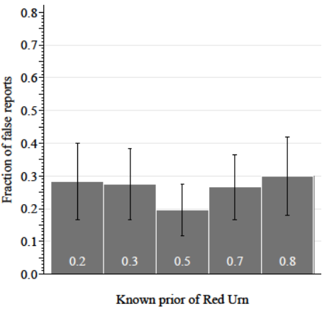
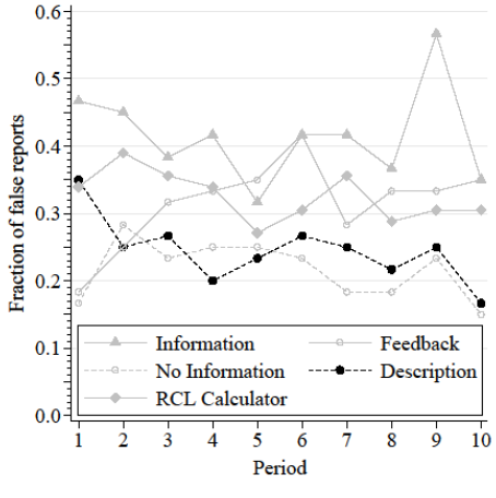
By round
By prior
False Reports
Summary
- Evidence for systematic distortions over objective priors
- When subjects are informed on the incentives they make systematic deviations
- That deviations are purposeful distortions is clearest
- But the environment is perhaps more artificial
- The same patterns are observed over Bayesian Posteriors
- Data here is harder to pinpoint as we don't know the 'true' posterior beliefs
- But distributions of response shift in same systematic way
- Two questions raised:
- Would this also hold for subjective beliefs?
- Does any of this matter for inference?
BSR Usage in Literature
- Most papers are eliciting probabilistic beliefs
- Most papers give two or more quantitative examples of the incentives
- Usage for beliefs is both as a LHS and RHS variable
EU assumption is used at observation level!
- EU in standard economic theory is typically used at an aggregate (i.e. average) level
- Predict a comparative static for a population
- But in the elicitation EU is used at the observation level:
- Use the IC under EU to interpret a choice over incentives as a measured belief
- 'Small' mistakes in the EU assumption can lead to a measurement error for any inference
- Regressions using mismeasured data can cause biased inference
Inferential Effects
To understand the effects on inference we use a simple model of the center-bias distortions
Observed belief is:
Regression model where X is a binary treatment indicator:
What happens when distorted beliefs are used?
Inferential Effects
Observed belief is:
Left-hand-side effect is clear:
- Mismeasurement of q leads to an attenuation of the estimated treatment effect
Inferential Effects
Observed belief is:
Right-hand-side treatment effect will depend on unknowns:
Niederle & Vesterlund (2006)
We return to the Niederle & Vesterlund study:
- Perform sums for a piece rate
- Perform sums in tournament
- Choose the preferred incentive
- Elicit subjective belief
- (here using BSR)
Run this study twice:
- NV-Information: Quantitative information
- NV-No-Information : No precise information
LHS: Confidence difference between men and women:
RHS: Competition difference for men and women after controlling for confidence:
NV Inference equations
Information predicted to attenuate gender confidence difference
Information predicted to make the gender-gap in tournament-entry larger (after controlling for confidence
Elicited Beliefs


NV-No-Information
NV-Information
Elicited Beliefs
NV-No-Information
NV-Information
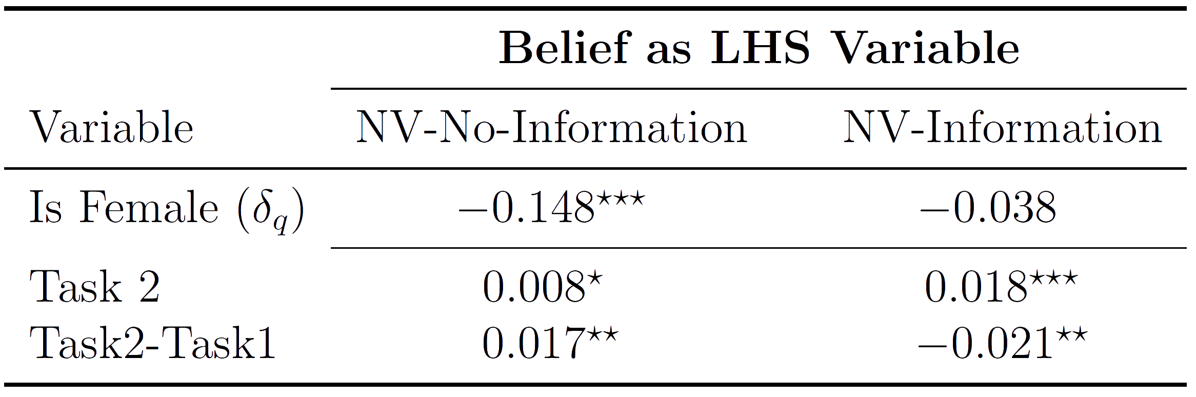
NV-Regressions LHS
Original finding is that:
- Women are less confident over their performance than men
- Prediction from model for NV-Information is that gender gap will move towards zero.
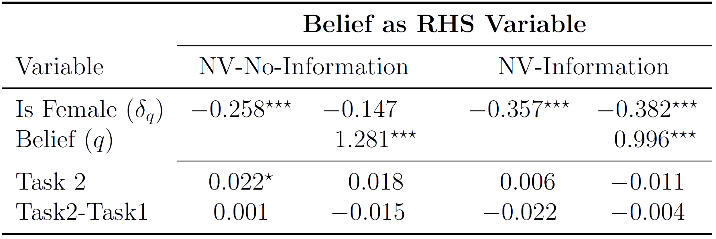
NV-Regressions RHS
- Original finding is that:
- Beliefs explain a significant proportion of the gender gap
- Prediction from model for NV-Information is that gender gap in competition is more negative:
- (gender gap in confidence)
- (Belief effect on entry)
NV Replication Results
- NV-Information distorts beliefs to center, relative to NV-No-Information
- This difference in the beliefs affects final inference:
- As a LHS variable it attenuates the treatment effect (here a gender gap over beliefs)
- As a RHS variable it widens the measured gender gap over competition after controlling for beliefs
- So, simply by providing the participants with information on the elicitation incentives, that we can qualitatively distort the subsequent inference
Going Forward...
- The BSR does not work as an incentive-compatible elicitation
- The less you tell the participants about the incentives, the worse the data
- This is true for:
- Objective priors
- Updated posteriors
- Subjective beliefs
- New elicitations are required. But how should we go about assessing them?
Propose two weak tests for behavioral incentive compatibility
- The mechanism should not yield worse data when participants are given precise information on the incentives on offer
- If presented with the pure incentives available in the mechanism, the majority of participants should be choosing the theorized maximizer
Weak Condition 1:
BIC Diagnostic 1:
- Information vs No Information comparison
Our paper demonstrates this methodology across:
- Elicitation of an objective prior
- Elicitation of an objective posterior
- Elicitation of a subjective belief
Have similar data showing this comparison for:
- Quadratic scoring rule
- Binarized-BDM
Weak Condition 2:
BIC Diagnostic 2:
- Extract the pure incentives from the elicitation and ask the participants to choose. A majority should be choosing the theorized maximizer
| Lottery pair | Red lottery ticket | Blue lottery ticket |
|---|---|---|
| A (0%) | 100% | 0% |
| B (10%) | 99% | 19% |
| C (20%) | 96% | 36% |
| D (30%) | 91% | 51% |
| E (40%) | 84% | 64% |
| F (50%) | 75% | 75% |
| G (60%) | 64% | 84% |
| H (70%) | 51% | 91% |
| I (80%) | 36% | 96% |
| J (90%) | 19% | 99% |
| K (100%) | 0% | 100% |
Fix the probability of Red and ask for a choice from:
Weak Condition 2:
We asked 120 subjects to choose their preferred lottery pair when the probability of Red was set to either 20% or 30%. Interpret choice via the EU assumption:


Weak Condition 2:
Same thing, but for QSR incentives:


Weak Condition 2:
Same thing, but for binarized-BDM (Karni)


Weak Condition 2:
First Price Auction, two bidders, uniform values:
\[v^\star=0.3\]
| Lottery pair | Prize | Probability |
|---|---|---|
| A (v=0.0) | $12 | 0% |
| B (v=0.1) | $10 | 10% |
| C (v=0.2) | $8 | 20% |
| D (v=0.3) | $6 | 30% |
| E (v=0.4) | $4 | 40% |
| F (v=0.5) | $2 | 50% |
| G (v=0.6) | $0 | 60% |
| H (v=0.7) | -$2 | 70% |
| I (v=0.8) | -$4 | 80% |
| J (v=0.9) | -$6 | 90% |
| K (v=1.0) | -$8 | 100% |
Weak Condition 2:
First Price Auction, two bidders, uniform values:
\[v^\star=0.7\]
| Lottery pair | Prize | Probability |
|---|---|---|
| A (v=0.0) | $28 | 0% |
| B (v=0.1) | $26 | 10% |
| C (v=0.2) | $24 | 20% |
| D (v=0.3) | $22 | 30% |
| E (v=0.4) | $20 | 40% |
| F (v=0.5) | $18 | 50% |
| G (v=0.6) | $16 | 60% |
| H (v=0.7) | $14 | 70% |
| I (v=0.8) | $12 | 80% |
| J (v=0.9) | $10 | 90% |
| K (v=1.0) | $8 | 100% |
Weak Condition 2:


\[v^\star =0.3\]
\[v^\star =0.7\]
First Price Auction:
Weak Condition 2:
Uniform Preferences
Correlated Preferences
Deferred Acceptance (Proposing over $6/$4/$2)
Assume all other players truthfully reveal
- Two other proposers
- Three prize amounts
Weak Condition 2:
Uniform Preferences
Deferred Acceptance (Proposing over $6/$4/$2)
| Lottery pair | $8 | $6 | $2 | $0 |
|---|---|---|---|---|
| A (6>8>2) | 26% | 64% | 10% | 0% |
| B (6>8>2) | 26% | 64% | 0% | 10% |
| C (6>2>8) | 10% | 64% | 26% | 0% |
| D (6>2) | 0% | 64% | 26% | 10% |
| E (8>6>2) | 64% | 26% | 10% | 0% |
| F (8>6) | 64% | 26% | 0% | 10% |
| G (8>2>6) | 64% | 10% | 26% | 0% |
| H (8>2) | 64% | 0% | 26% | 10% |
| I (2>6>8) | 10% | 26% | 64% | 0% |
| J (2>6) | 0% | 26% | 64% | 10% |
| K (2>8>6) | 26% | 10% | 64% | 0% |
| L (2>8) | 26% | 0% | 64% | 10% |
Weak Condition 2:
Correlated Preferences
Deferred Acceptance (Proposing over $6/$4/$2)
| Lottery pair | $8 | $6 | $2 | $0 |
|---|---|---|---|---|
| A (6>8>2) | 9% | 64% | 29% | 0% |
| B (6>8) | 9% | 64% | 0% | 29% |
| C (6>2>8) | 1% | 64% | 36% | 0% |
| D (6>2) | 0% | 64% | 36% | 1% |
| E (8>6>2) | 41% | 33% | 26% | 0% |
| F (8>6) | 41% | 33% | 0% | 26% |
| G (8>2>6) | 41% | 7% | 52% | % |
| H (8>2) | 47% | 0% | 52% | 7% |
| I (2>6>8) | 1% | 8% | 91% | 0% |
| J (2>6) | 0% | 8% | 91% | 1% |
| K (2>8>6) | 2% | 7% | 91% | 0% |
| L (2>8) | 2% | 0% | 91% | 7% |
Weak Condition 2:
Uniform Preferences
Correlated Preferences
Deferred Acceptance (Proposing over $6/$4/$2)


Conclusions
- On the Binarized Scoring Rule
- Substantial false-report rate for objective prior
- Systematic deviations driven by information on the incentives
- Between (Information vs No Information)
- Within (gradual Feedback)
-
Distortions generated can qualitatively affect inference
-
Replication of Niederle & Vesterlund fails when incentive information present
-
Conclusion
- Overly content to appeal to theoretical incentive compatibility, when what is actually required are notions of behavioral compatibility
- For belief elicitation, qualitative notions are effective:
- Both No Information and Description work well
- But need to ask ourselves if it truly the incentives, instead of framing/call to authority
- Might want to ask if it even makes sense to collect arbitrarily precise beliefs.
- Methodology offers simply diagnostic checks for behavioral incentive compatibility
- Simple demonstrations for check on First Price auctions and Matching mechanisms