Misspecificaiton & Effect Size
Experimenter Demand Effects
UC Dublin ReCLAIM, June 2026

David
Danz

Guillermo
Lezama
Amazon

Pun
Winichakul
Smith College

Priyoma
Mustafi
Ahmedabad

Marissa
Lepper
Texas A&M

Lise
Vesterlund
Pittsburgh

Alistair
Wilson
Pittsburgh
UC Dublin, June 2026
Guillermo
Lezama
Amazon
Pun
Winichakul
Smith College
David
Danz
Priyoma
Mustafi
Ahmedabad
Marissa
Lepper
Texas A&M
Lise
Vesterlund
Pittsburgh
Alistair
Wilson
Pittsburgh
Misspecificaiton & Effect Size
Experimenter Demand Effects
Experimenter Demand
[The participant’s] general attitude of mind is that of ready complacency and cheerful willingness to assist the investigator in every possible way by reporting to him those very things which he is most eager to find.
-A H. Pierce, 1908
The subject’s performance in an experiment might almost be conceptualized as problem-solving behavior... he sees it as his task to ascertain the true purpose of the experiment and respond in a manner which will support the hypotheses being tested.
-M. T. Orne, 1962
Experimenter Demand
the critical assumption underlying the interpretation of data from lab experiments is that the insights gained can be extrapolated to the world beyond-S. Levitt and J. List, 2007
many reasons to suspect that these laboratory findings might fail to generalize to real markets
-S. Levitt and J. List, 2008

Jonathan
de Quidt
Queen Mary
Lise
Vesterlund
Pittsburgh
Alistair
Wilson
Pittsburgh
Experimenter Demand
2019 (ed. Schram & Ule)
2026 (ed. Rees-Jones)
Impact of EDE on Inference?
-
The objective of much of experimental research is qualitative inference (Kessler & Vesterlund, 2015).
-
Causal effect of \(X\) on \(Y\)
-
Direction and economically meaningful (and statistically significant)
-
-
Can EDE alter inference?
-
Impact of an ill-intentioned experimenter who differentially applies positive and negative demand across a decision pair?
-
False negatives – where true effect is positive
-
False positives – where true effect is null
-
-
Outline
3. Effect Size in Economics
2. Effect Size across Populations
1. EDE Measurment
What do we do?
- Use “worst case scenario” to assess false negatives and false positives
- Differentially apply strong positive and negative demand across a treatment/control decision pair (de Quidt, Haushofer and Roth, AER 2018)
You will do us a favor if you take a higher (lower) action than you normally would.
- Four core domains in Behavioral Economics
- Probability weighting
- The Endowment effect
- Charitable giving
- Intertemporal choice
- Seven behavioral comparative statics
(Risk)
(Ownership)
(Self vs. Other)
(Now vs Later)
Design
- Eight within-subject decisions:
- Four lottery valuations:
- WTP and WTA
- Lotteries with 10% and 90% chance of winning $10
- Two donations:
- Matched (low cost)
- Unmatched (high cost)
- Two intertemporal allocations:
- Immediate (today vs a week from now)
- Delayed (tomorrow vs week from tomorrow)
- Four lottery valuations:
Design
- Eight within-subject decisions:
- Four lottery valuations
- Two donations
- Two intertemporal allocations
- Three between-subject treatments:
- No demand
- Positive demand
- Negative demand
- Three Populations:
- Laboratory (Pitt undergrads)
- Mechanical Turk
- Prolific
Online Populations

Papers on Google Scholar
2013
2023
2018
Design
- Eight within-subject decisions:
- Four lottery valuations
- Two donations
- Two intertemporal allocations
- Three between-subject treatments:
- No demand
- Positive demand
- Negative demand
- Three Populations:
- Laboratory (Pitt undergrads)
- Mechanical Turk
- Prolific
(N=236, ~80/treatment)
(N=756, ~250/treatment)
(N=732, ~240/treatment)
Endowment Effect
Endowment Effect
Literature Predictions:
- Kahneman, Knetsch and Thaler (1990; 1991)
- \( \text{WTA}( \tfrac{1}{10} ) > \text{WTP}( \tfrac{1}{10} ) \)
- \( \text{WTA}( \tfrac{9}{10} ) > \text{WTP}( \tfrac{9}{10} ) \)
Task:
WTA: endowed with $10 and lottery, asked about willingness to accept a price for lottery.
WTP: Endowed with $10 and asked about willingness to pay a price for the lottery
Endowment Effect

\(p<0.001\)
Endowment Effect

\(p=0.002\)
Endowment Effect

\(p<0.001\)
You will do us a favor if you indicate a lower willingness to [buy] than you normally would
Endowment Effect

\(p<0.001\)
You will do us a favor if you indicate a higher willingness to [buy] than you normally would
Endowment Effect

\(p=0.012\)
This is extreme differential demand over the comparative static
Endowment Effect (High)

\(p=0.019\)
Endowment Effect (High)

\(p=0.731\)
Endowment Effect (High)

\(p=0.001\)
Endowment Effect (High)

\(p=0.127\)
Different Populations
Sensitivities

Lab

MTurk

Prolific
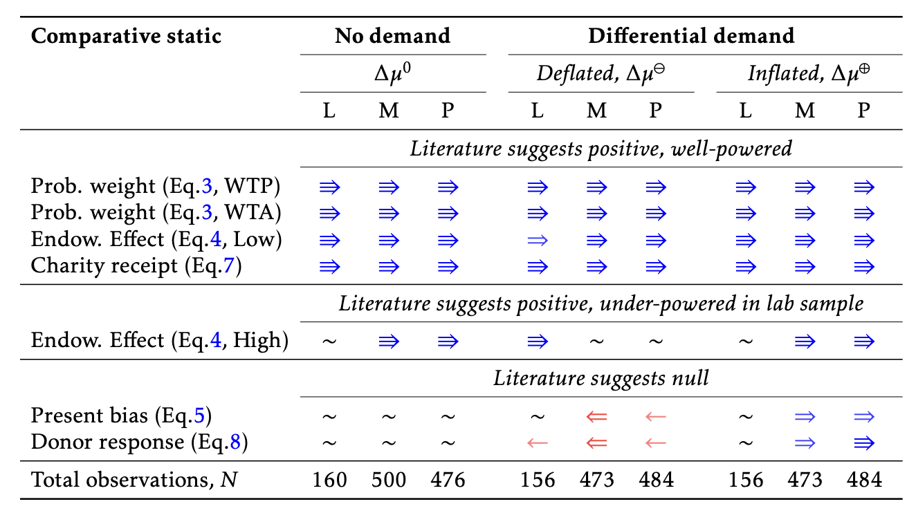
False Positive in Online Samples
- All of the domains where we expect a directional result are replicated online:
- Probability Weighting
- Endowment effect (low probs)
- Charitable giving
- However, we do find that extreme experimenter demand can create false positives in both online samples:
- Present Bias
- Charitable giving foregone amount
- Reasons:
- Slightly more consistent demand effects in online sample
- Larger sample sizes easier to generate significance
- With large samples, need to focus on economic size of the effects!
False Positive in Online Samples
Present Bias
Task:
Convex budget set. Have $10 to be paid at date \(t\), can move up to $9 to date \(t+7\) earning 20% interest on moved amount. Treatments are for:
- \(t=0\) (today vs week from today)
- \(t=1\) (tomorrow vs week from tomorrow)
Literature Predictions:
- Andreoni and Sprenger, 2012:
- Compared to an immediate sooner date, participants will be no more patient when the sooner date is delayed
- Purposeful null result: \( \text{Transfer}(t=0) = \text{Transfer}(t=1) \)
False Positive in Online Samples

Present Bias: Laboratory sample
False Positive in Online Samples

Present Bias: MTurk sample
False Positive in Online Samples

Present Bias: MTurk sample
\(p=0.039\)
False Positive in Online Samples

Present Bias: MTurk sample
\(p=0.033\)
False Positive in Online Samples

Present Bias: Prolific sample
False Positive in Online Samples

Present Bias: Prolific sample
\(p=0.043\)
False Positive in Online Samples

Present Bias: Prolific sample
\(p=0.112\)
Effect size normalization
- For each comparative static we construct a normalized effect size \[ y_i = \hat{\beta_0} +\hat{\beta}_1\cdot 1_{\text{Treat}}+\hat{\epsilon}_i \]
- Variation normalized coefficient is: \[\hat{D}=\frac{\hat{\beta}_1}{\hat{\sigma}_{\hat{\epsilon}}} \]
- This effect size statistic is what is referred to as Cohen's-\(D\)
- Cohen gives the informal guidance that \(0.2\sigma\) is small, \(0.5\sigma\) medium, \(0.8\sigma\) large
- This effect size statistic is what is referred to as Cohen's-\(D\)
- So interpretation of effect size is as a multiple of the unexplained variation over the decision \(y\) (separate from the treatment effect)
- Many inferences require conditioning on more variables
- Here if the total data size is \(N\), then we can just think of \(\sqrt{N}\cdot\hat{D}\) as the two-sample Student's-\(t\) test statistic
Comparative Statics as \(D\)'s

Comparative Static as \(D\)'s

Relation to Significance
- For each comparative static we construct a normalized effect size \[ y_i = \hat{\beta_0} +\hat{\beta}_1\cdot 1_{\text{Treat}}+\hat{\epsilon}_i \]
- Variation normalized coefficient is: \[\hat{D}=\frac{\hat{\beta}_1}{\hat{\sigma}_{\hat{\epsilon}}} \]
- Here if the total data size is \(N\), then we can just think of \(\sqrt{N}\cdot\hat{D}\) as the two-sample Student's-\(t\) test statistic
Comparative Static Sensitivity

Effect Sizes
- Our evidences suggests even extreme experimenter demand (strong and differential across treatment) can push comparative statics by approximately \(0.2\sigma\)
- How big are effects sizes in experimental studies?
- Initial stages of data synthesis for 33 experimental studies in the AER in the last seven years:
- Available data
- "Important" general-interest studies
- For each paper we try to construct a simple normalized effect size \[ y_i = \hat{\beta_0} +\hat{\beta}_1\cdot 1_{\text{Treat}}+\hat{\epsilon}_i \]
- We generalize this approach for Diff-in-Diff designs to focus on the interaction
- Normalized coefficient is: \[\hat{D}=\frac{\hat{\beta}_1}{\hat{\sigma}_{\hat{\epsilon}}} \]
Effect Sizes

Effect Sizes

Effect Sizes

Effect Sizes (Non-null)

Effect Sizes

Effect Sizes

Effect Sizes

Conclusions
- Limited EDE impact on inference:
- For four classic domains EDE bounds narrow for lab and online
- Highly comparable normalized effect sizes across populations
- Potential impact of ill-intentioned experimenter:
- Lab: no false negatives or false positives for typical sample sizes
- Online: no false negatives, but false positives (small)
- Results from sample of AER papers:
- Typical effect sizes in economics are substantial, beyond what we can obtain with experimenter demand
- Reporting externally comparable measures of effect can help clarify where we might/might not be concerned with EDE/misspecification for qualitative effects.
Probability Weighting
Probability Weighting
Literature Predictions:
- Kahneman & Tversky 1979; Prelec 1998
- Risk seeking at low probabilities: \(\text{WTP}(\tfrac{1}{10})>\$1)\)
- Risk averse at high probabilities: \(\text{WTP}(\tfrac{9}{10})<\$9)\)
Task:
Endowed with $10, and asked about willingness to pay for the lottery:
\( p\cdot\$10\oplus(1-p)\cdot \$0\)
with two probabilities of winning \(p\in\left\{\tfrac{1}{10},\tfrac{9}{10}\right\}\)
Probability Weighting

\(p<0.001\)
\(p<0.001\)
Probability Weighting

\(p=0.002\)
\(p<0.001\)
Probability Weighting

You will do us a favor if you indicate a lower willingness to buy than you normally would
\(p<0.001\)
\(p<0.001\)
Probability Weighting

You will do us a favor if you indicate a higher willingness to buy than you normally would
\(p<0.001\)
\(p<0.001\)
Probability Weighting

This is extreme and differential demand over the comparative static
\(p<0.001\)
\(p<0.001\)
Charitable Giving
Chartiable Giving
Task:
Endowed with $20, and given the option to donate any of this to a local Children's Hospital. Donation cost is either Low (matched donation, \(c=\$0.50\)) or High (unmatched donation, \(c=\$1.00\)).
Literature Predictions:
- Andreoni & Miller (2002); Huck & Rasul, (2011); Karlan & List, (2007)
- Charity receives larger donation with than without a match
- DonatedAmount(Low)>DonatedAmount(High)
- Charity receives larger donation with than without a match

\(p<0.001\)
Present Bias
Present Bias
Task:
Convex budget set. Have $10 to be paid at date \(t\), can move up to $9 to date \(t+7\) earning 20% interest on moved amount. Treatments are for:
- \(t=0\) (today vs week from today)
- \(t=1\) (tomorrow vs week from tomorrow)
Literature Predictions:
- Andreoni and Sprenger, 2012:
- Compared to an immediate sooner date, participants will be no more patient when the sooner date is delayed
- Purposeful null result: \( \text{Transfer}(t=0) = \text{Transfer}(t=1) \)
Present Bias
\(p=0.339\)
Present Bias

\(p=0.239\)
Present Bias

\(p=0.465\)
Present Bias

\(p=0.819\)
Sensitivities
Lab:
\(p=0.304\) from Fisher's exact on directions
Sensitivities
Mturk:
\(p=0.020\) from Fisher's exact on directions
Sensitivities
Prolific:
\(p=0.003\) from Fisher's exact on directions