Calculating properties in AFQMC using automatic differentiation
Properties in AFQMC
- Mixed estimators often require very accurate trials
- Backpropagation correlates bra and ket to reduce noise
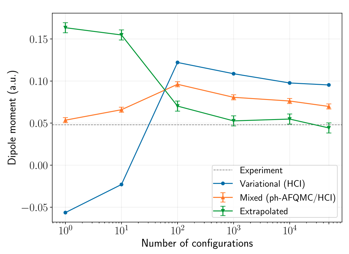
- Variational estimators are tricky to evaluate in AFQMC
- Analytical derivatives (?)
- Finite difference:
Response formulation
- small energy differences between large noisy energies \(\rightarrow\) correlated sampling
- Lots of calculations required if multiple observables or forces are desired
- Automatic differentiation is a viable alternative
Outline
- Forward and reverse mode automatic differentiation:
putting the chain rule to good use
- Analysis of stochastic and systematic errors:
scaling of error and cost with system and basis size
- Results:
comparison to experimental dipole moments
Automatic differentiation (AD)
Consider a program that evaluates a function \(f\)
Intermediates formed during execution
The Jacobian vector products are performed numerically
The order in which these evaluations are performed depends on the problem and dictates efficiency
Forward mode
Suppose we only want derivatives wrt a small number of inputs

derivative time cost ~ 2-3 \(\times\) cost of \(f\)
Good choice if only a small number of observables are required
Reverse mode
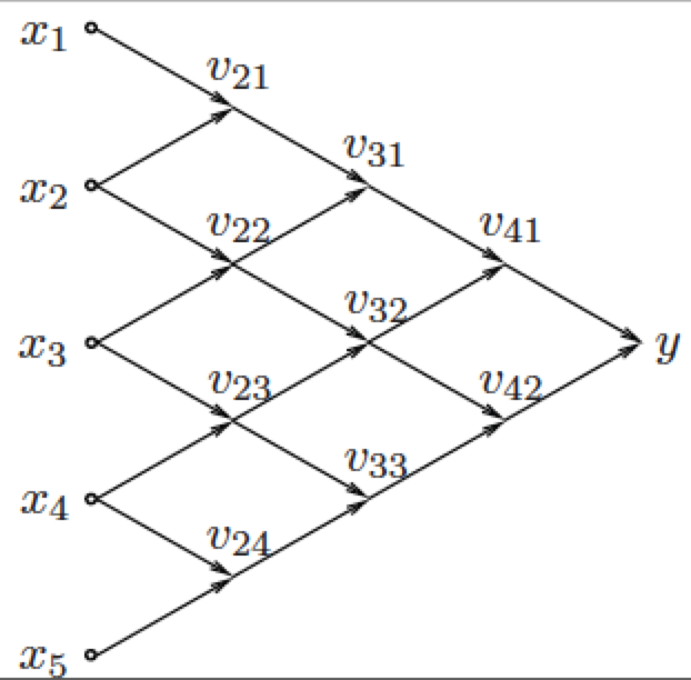
To calculate derivatives of few outputs wrt to a lot of inputs

gradient time cost ~ 2-4 \(\times\) cost of \(f\)
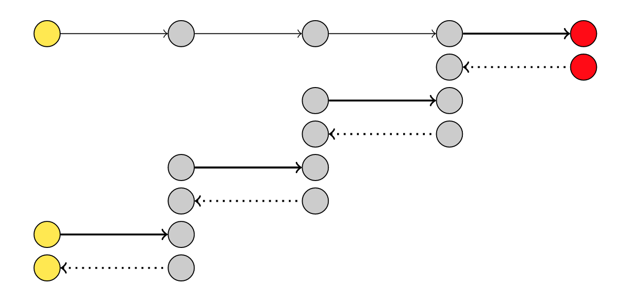
checkpointing to reduce memory cost
Suitable for RDM's e.g.
Toy example
Harmonic oscillator in an electric field VMC:
Correlated sampling 1:
Correlated sampling 2:
Use the same random numbers in \(E(\delta)\) and \(E(0)\) calculations,
FD equivalent of AD
Possibility of divergences in correlated sampling \(\rightarrow\) AD?
Assaraf, Caffarel, Kollias '11
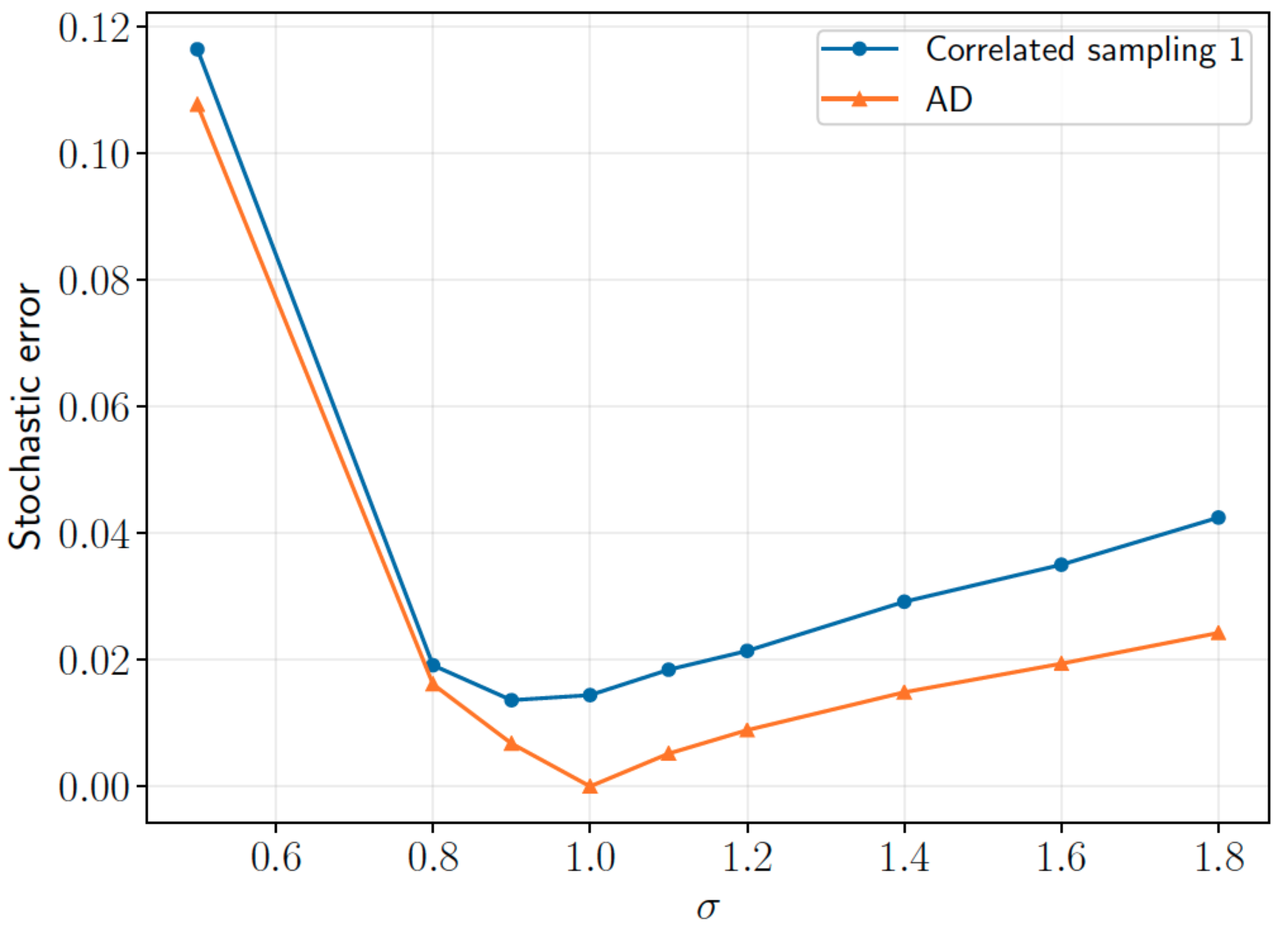
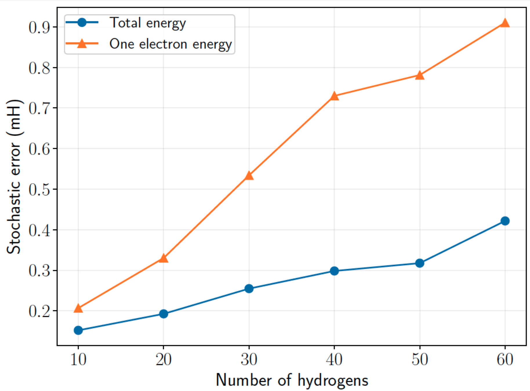
Scaling of stochastic error in H chains (minimal basis)
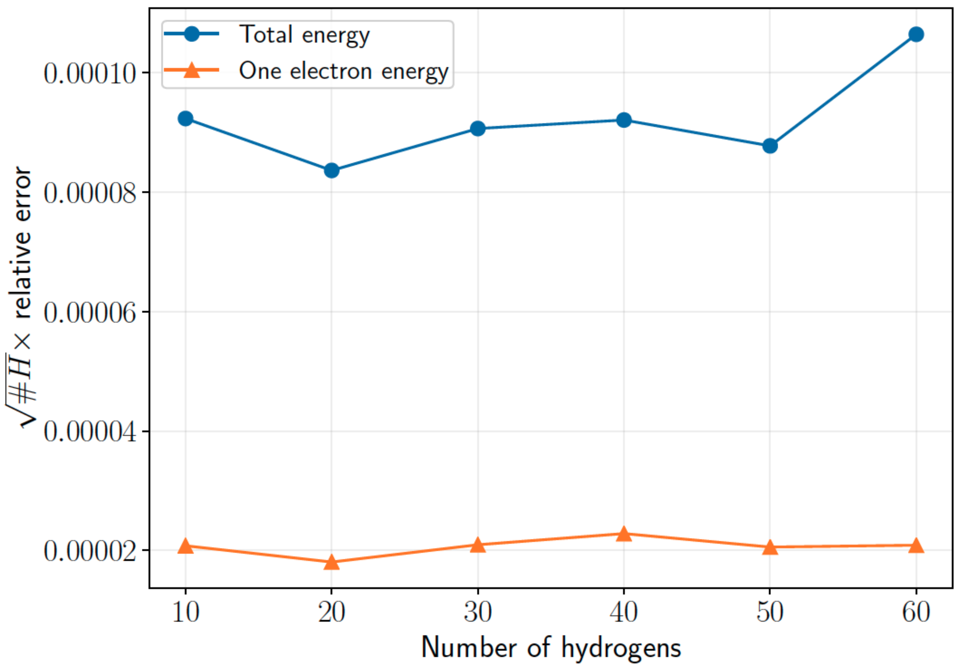
Relative error
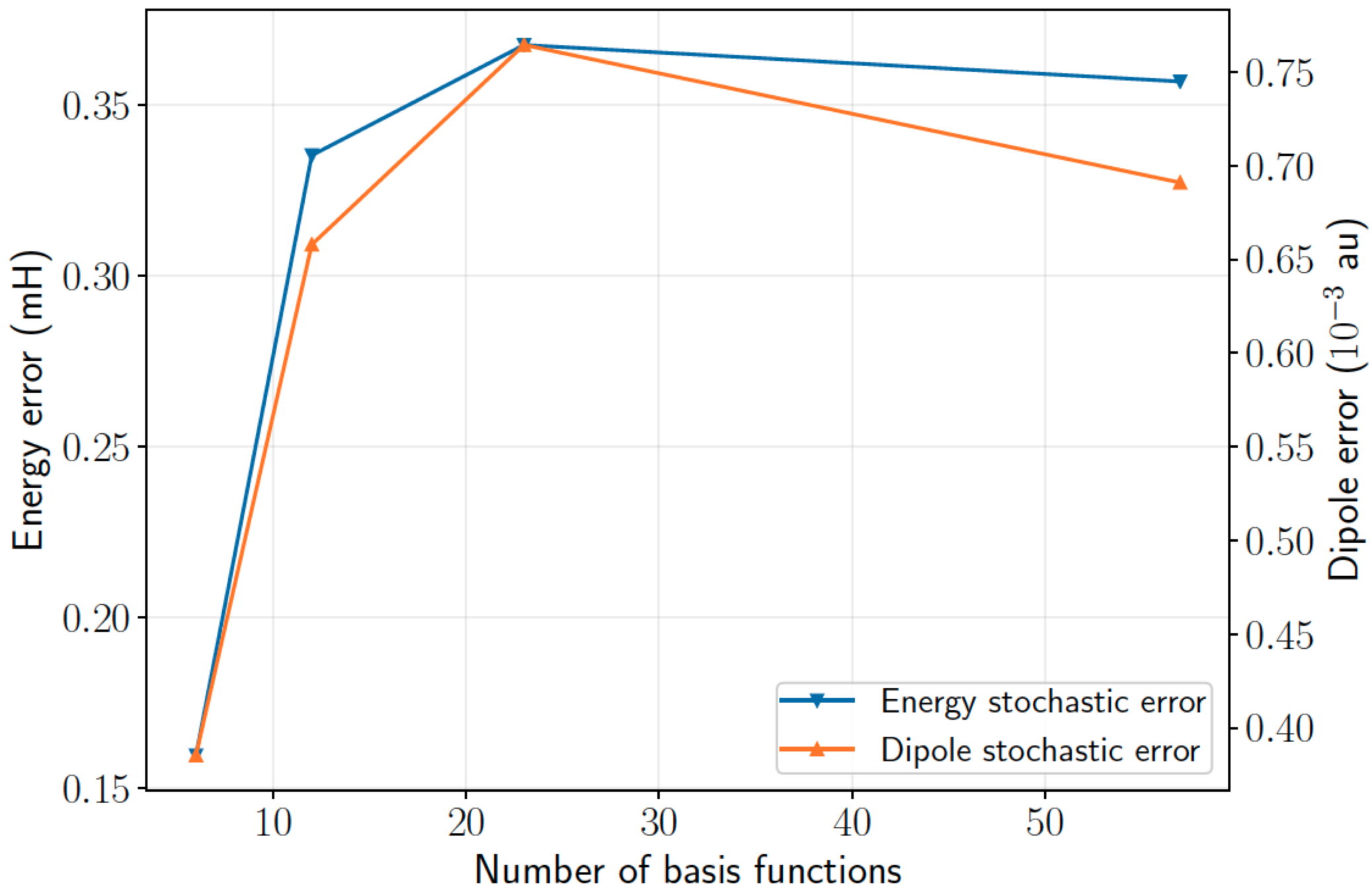
Scaling of error with basis size in water
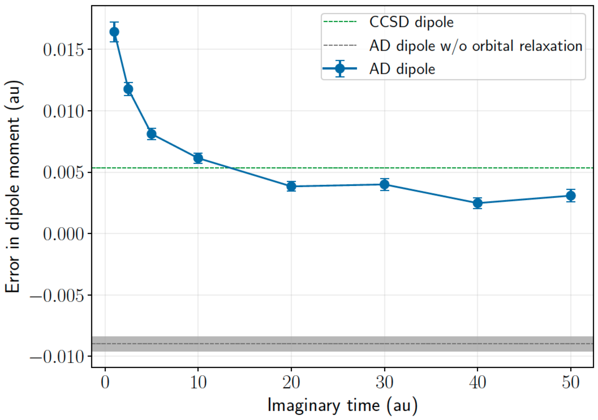
Systematic errors in ammonia dipole moment (dz basis)
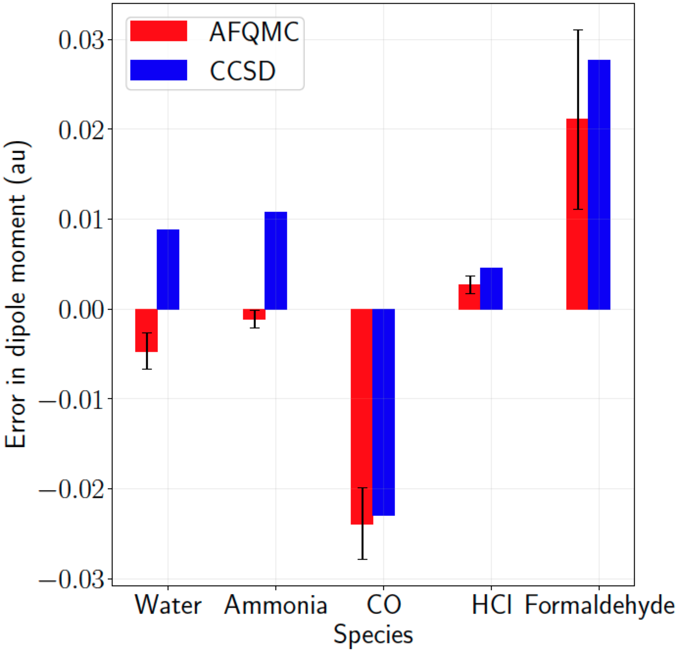
Dipole moments in the continuum limit
Self-consistent AFQMC to improve properties
AFQMC reverse AD 1RDM \(\rightarrow\) natural orbitals for trial
Test for CO (in DZ basis):
CCSD(T) dipole: 0.087
AFQMC dipole without self-consistency: 0.073(4)
AFQMC dipole with self-consistency: 0.093(3)
Energy improved by about ~2m mH as well!
Summary
AD with AFQMC brings observable calculations on par with energy calculations
Forward and reverse AD can be employed depending on the problem
Higher order properties, nuclear forces, ...