Challenging electronic structure problems

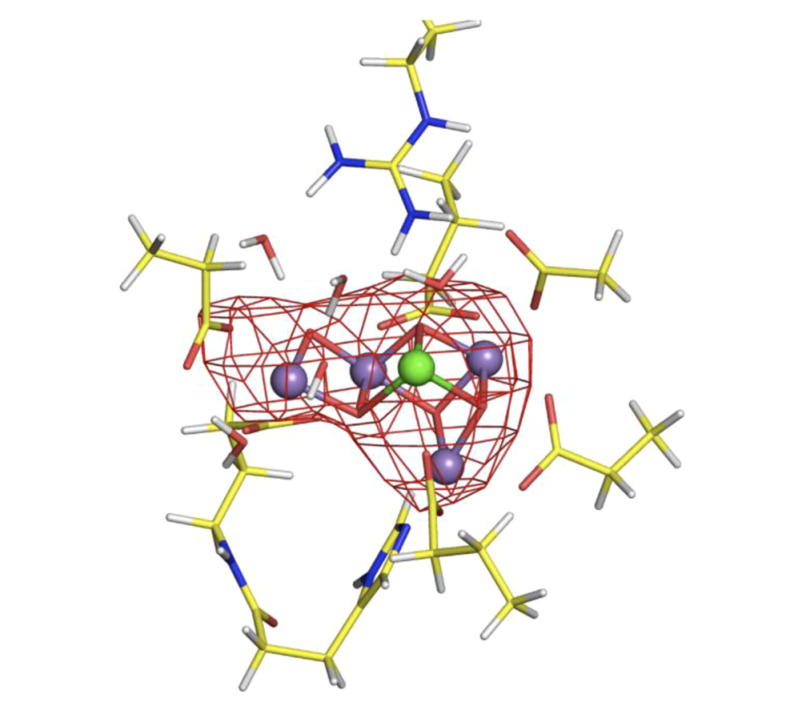
oxygen evolving complex (photosynthesis)

Cluster models of metalloenzymes

$[\text{Mn}_4\text{CaO}_5]$

$[\text{Cu}_2\text{O}_2]$

tyrosinase

(melanin production)

Example: $[\text{Cu}_2\text{O}_2]^{2+}$ isomerization

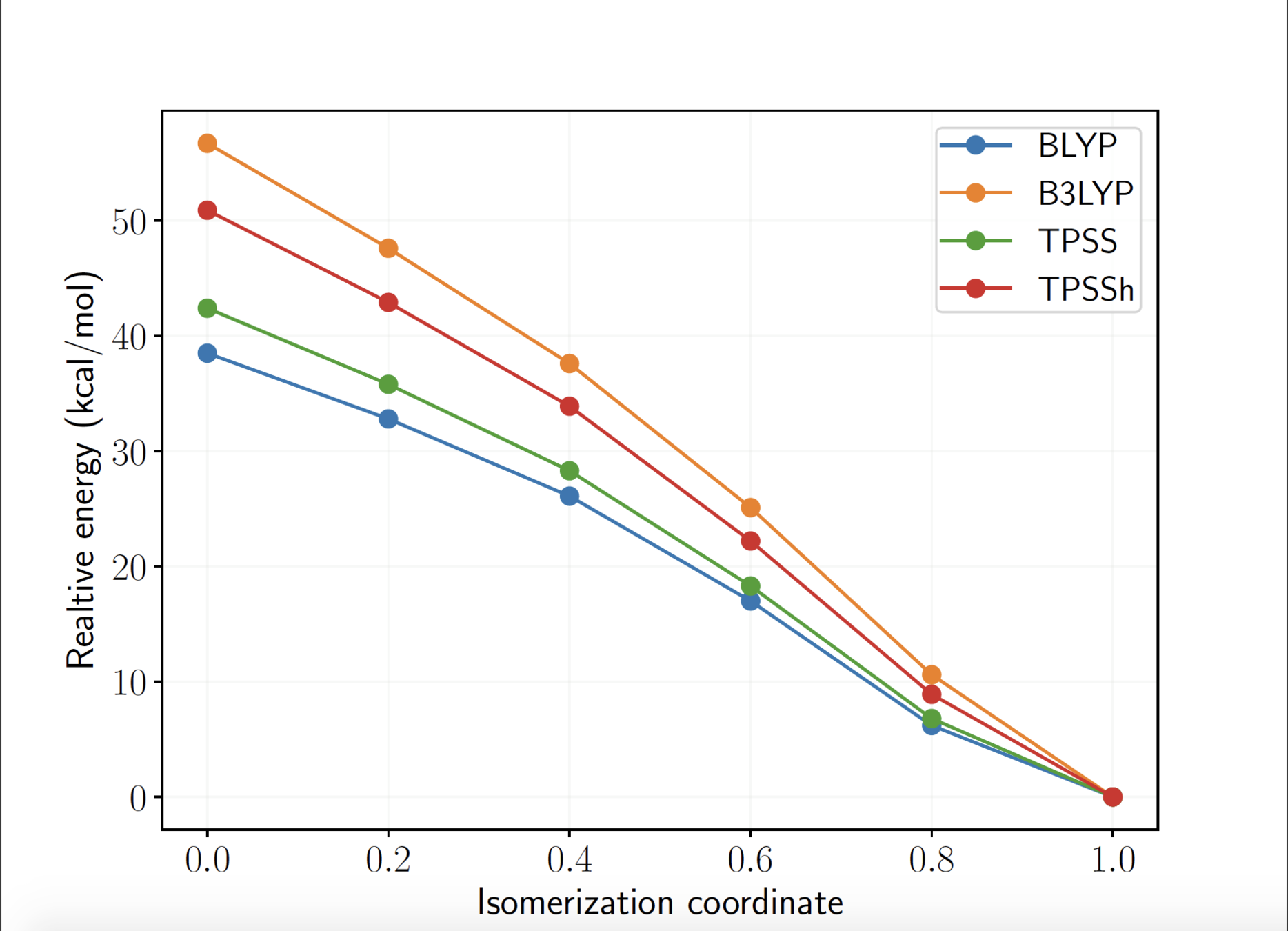
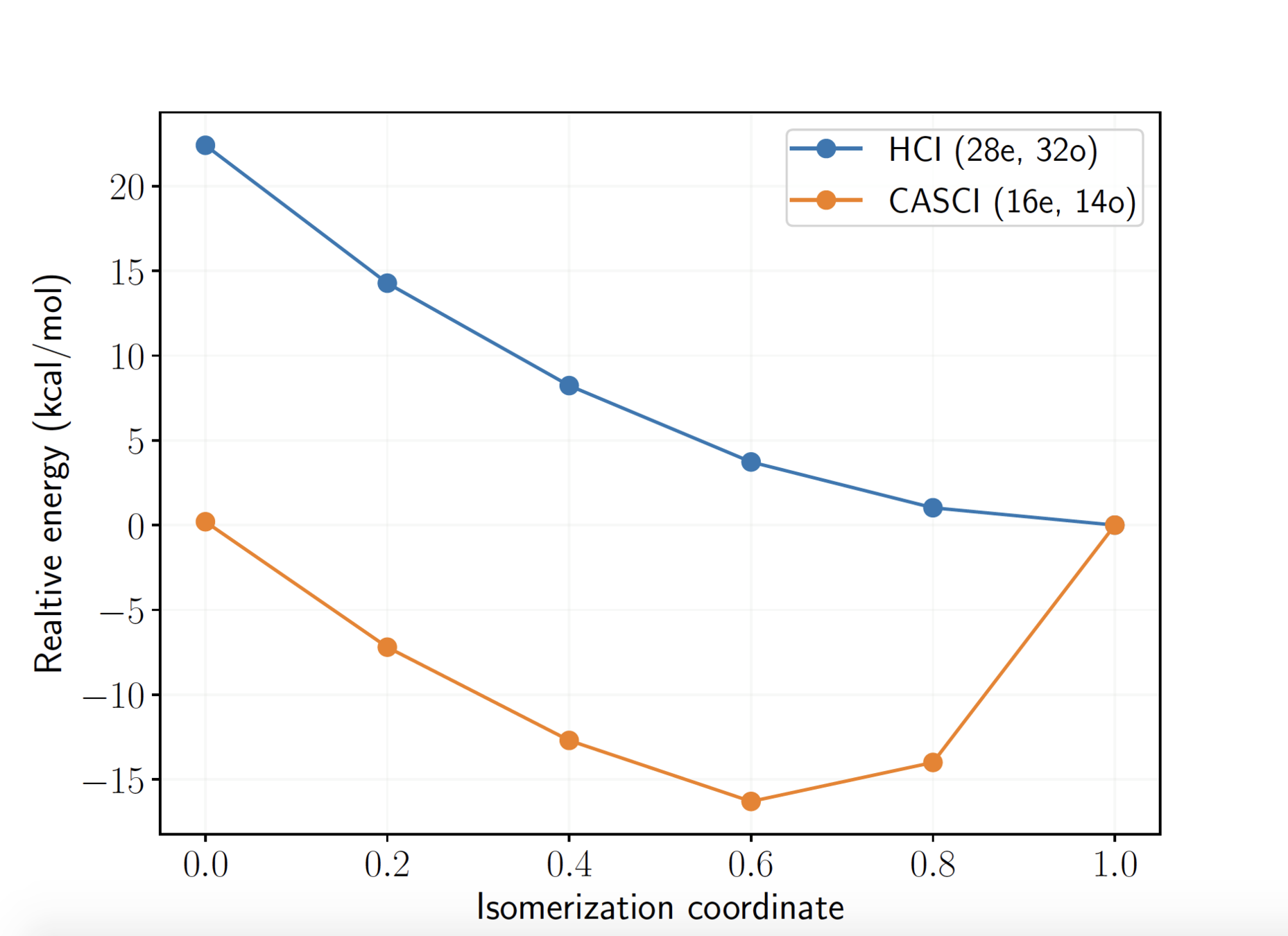
DFT: large differences in relative energies depending on the functional

Active space wave functions: (28e, 32o) includes Cu 3d, 4d, and O 2p, 3p orbitals, Hilbert space dimension: $10^{17}$ !

Cramer et al. J. Phys. Chem. A 2006, 110, 1991-2004

arXiv:2008.00220

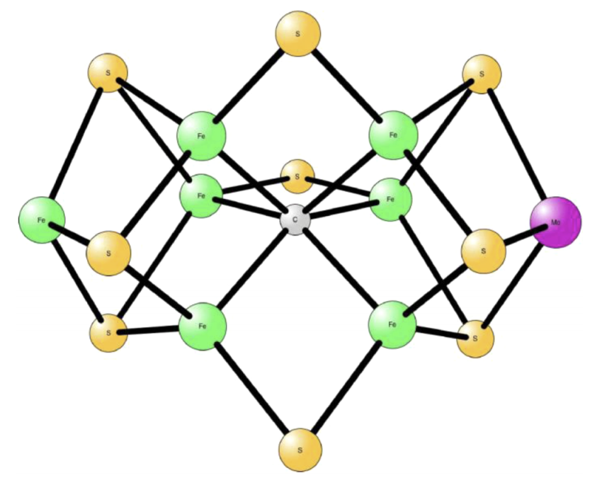
Nitrogenase FeMo cofactor

7 iron atoms, 1 molybdenum atom

Local and canonical descriptions

\hat{H} = -\sum_{\langle ij\rangle,\sigma}(\hat{a}_{i\sigma}^{\dagger}\hat{a}_{j\sigma}+\hat{a}_{j\sigma}^{\dagger}\hat{a}_{i\sigma}) + U\sum_i\hat{n}_{i\uparrow}\hat{n}_{i\downarrow}

\hat{H} = -\sum_{\langle ij\rangle,\sigma}(\hat{a}_{i\sigma}^{\dagger}\hat{a}_{j\sigma}+\hat{a}_{j\sigma}^{\dagger}\hat{a}_{i\sigma}) + U\sum_i\hat{n}_{i\uparrow}\hat{n}_{i\downarrow}

Hubbard:

hopping (kinetic energy)

onsite e-e repulsion

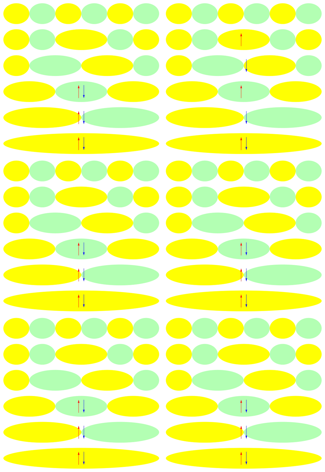
Ground state of half-filled 1-D 6 site model: U = 1

$x$

$E$

Efficient description using delocalized canonical orbital configurations:

|\psi\rangle= |\phi_0\rangle + \sum_i c_i\hat{E}_i|\phi_0\rangle

|\psi\rangle= |\phi_0\rangle + \sum_i c_i\hat{E}_i|\phi_0\rangle

Hartree-Fock reference

particle hole excitations

Ground state of half-filled 1-D 6 site model: U = 10

Local and canonical descriptions

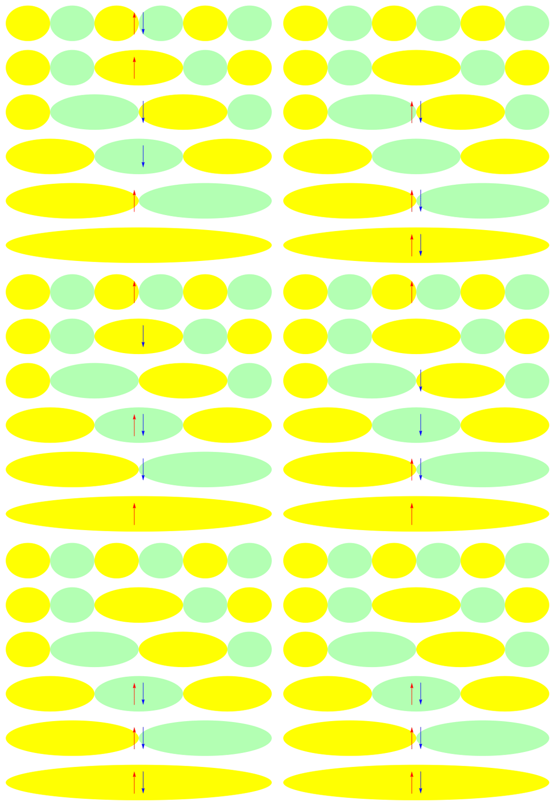
Efficient description with a Jastrow factor using local orbitals:

|\psi\rangle = \exp\left(\sum J_{ij}\hat{n}_i\hat{n}_j\right)|\phi_0\rangle

|\psi\rangle = \exp\left(\sum J_{ij}\hat{n}_i\hat{n}_j\right)|\phi_0\rangle

Jastrow

HF ref.

Correlation by penalizing local charge fluctuations

Combining Jastrow with multi-Slater: Jastrow encodes strong interactions, while multi-Slater captures weak and more general interactions, like exchange

|\psi\rangle = \exp\left(\sum J_{ij}\hat{n}_i\hat{n}_j\right) \sum_i c_i|\phi_i\rangle

|\psi\rangle = \exp\left(\sum J_{ij}\hat{n}_i\hat{n}_j\right) \sum_i c_i|\phi_i\rangle

|\phi_i\rangle = \prod \hat{C}_t^{\dagger}\hat{C}_p|\phi_0\rangle

|\phi_i\rangle = \prod \hat{C}_t^{\dagger}\hat{C}_p|\phi_0\rangle

Variational principle

Energy of any "valid" wave function is an upper bound for the ground state energy:

E[\psi]=\dfrac{\langle\psi|\hat{H}|\psi\rangle}{\langle\psi|\psi\rangle}\geq E_0

E[\psi]=\dfrac{\langle\psi|\hat{H}|\psi\rangle}{\langle\psi|\psi\rangle}\geq E_0

To find an approximation to the ground state wave function:

Start with a wave function parametrization: Jastrow multi-Slater
Calculate energy: we use variational Monte Carlo (VMC) to perform a random walk in the space of local orbital electronic configurations:

E[\psi] = \langle E_L\rangle,\quad E_L[n] = \dfrac{\langle n|\hat{H}|\psi\rangle}{\langle n|\psi\rangle}

E[\psi] = \langle E_L\rangle,\quad E_L[n] = \dfrac{\langle n|\hat{H}|\psi\rangle}{\langle n|\psi\rangle}

Vary parameters to minimze energy: difficult nonlinear optimization

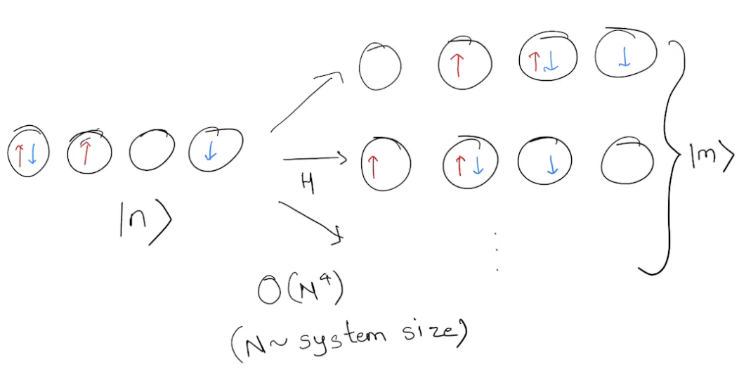
local energy of walker $|n\rangle$

Local energy of Jastrow multi-Slater

The local energy is given by

\dfrac{\langle n|\hat{H}|\psi\rangle}{\langle n|\psi\rangle}=\sum_m\langle n|\hat{H}\hat{\mathcal{J}}|m\rangle\sum_ic_i\dfrac{\langle m|\phi_i\rangle}{\langle n|\psi\rangle},

\dfrac{\langle n|\hat{H}|\psi\rangle}{\langle n|\psi\rangle}=\sum_m\langle n|\hat{H}\hat{\mathcal{J}}|m\rangle\sum_ic_i\dfrac{\langle m|\phi_i\rangle}{\langle n|\psi\rangle},

\hat{H} = \sum h_{ia}\hat{L}_a^{\dagger}\hat{L}_{i}+\sum v_{ijab}\hat{L}^{\dagger}_a\hat{L}_b^{\dagger}\hat{L}_j\hat{L}_i

\hat{H} = \sum h_{ia}\hat{L}_a^{\dagger}\hat{L}_{i}+\sum v_{ijab}\hat{L}^{\dagger}_a\hat{L}_b^{\dagger}\hat{L}_j\hat{L}_i

Sum of $N_c$ such terms for each $|m\rangle$ . Since there are $O(N^4)$ $|m\rangle$ , this is expensive.

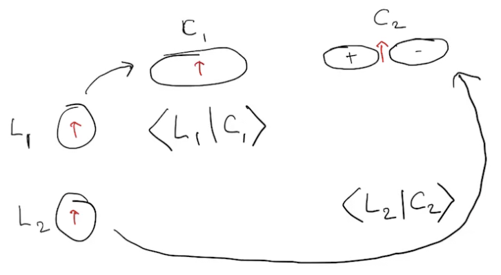
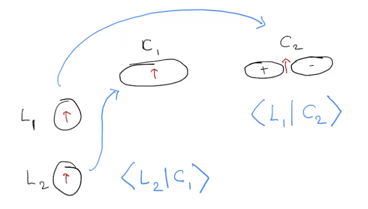
\langle m|\phi_i\rangle = \langle n|\prod \hat{L}_i^{\dagger}\hat{L}_a\prod \hat{C}_t^{\dagger}\hat{C}_p|\phi_0\rangle

\langle m|\phi_i\rangle = \langle n|\prod \hat{L}_i^{\dagger}\hat{L}_a\prod \hat{C}_t^{\dagger}\hat{C}_p|\phi_0\rangle

What is the overlap between a local configuration and a canonical one?

$\hat{L}$ : local, $\hat{C}$ : canonical

Overlaps are determinants

$\langle L_1L_2|C_1C_2\rangle =$ Amplitude of $|L_1L_2\rangle\rightarrow|C_1C_1\rangle$

Two ways to accomplish this:

or

$L_1\rightarrow C_1$ and $L_2\rightarrow C_2$ : $\langle L_1|C_1\rangle \times \langle L_2|C_2\rangle$

$L_1\rightarrow C_2$ and $L_2\rightarrow C_1$ : $\langle L_1|C_2\rangle \times \langle L_2|C_1\rangle$

\langle L_1L_2|C_1C_2\rangle = \langle L_1|C_1\rangle \langle L_2|C_2\rangle - \langle L_1|C_2\rangle \langle L_2|C_1\rangle = \det\begin{pmatrix} \langle L_1|C_1\rangle & \langle L_1|C_2\rangle\\ \langle L_2|C_1\rangle & \langle L_2|C_2\rangle\\ \end{pmatrix}

\langle L_1L_2|C_1C_2\rangle = \langle L_1|C_1\rangle \langle L_2|C_2\rangle - \langle L_1|C_2\rangle \langle L_2|C_1\rangle = \det\begin{pmatrix} \langle L_1|C_1\rangle & \langle L_1|C_2\rangle\\ \langle L_2|C_1\rangle & \langle L_2|C_2\rangle\\ \end{pmatrix}

fermion antisymmetry

Cost of calculating $N\times N$ determinant: $O(N^3)$

Generalized Wick's theorem

\dfrac{\langle n|\hat{L}_i^{\dagger}\hat{L}_a|\phi_0\rangle}{\langle n|\phi_0\rangle}=G^L_{ai},

\dfrac{\langle n|\hat{L}_i^{\dagger}\hat{L}_a|\phi_0\rangle}{\langle n|\phi_0\rangle}=G^L_{ai},

Green's function,

involves calculating inverse ( $O(N^3)$ )

\dfrac{\langle n|\hat{L}_i^{\dagger}\hat{L}_a\hat{L}^{\dagger}_j\hat{L}_b|\phi_0\rangle}{\langle n|\phi_0\rangle}=G^L_{ai}G^L_{bj}-G^L_{aj}G^L_{bi}

\dfrac{\langle n|\hat{L}_i^{\dagger}\hat{L}_a\hat{L}^{\dagger}_j\hat{L}_b|\phi_0\rangle}{\langle n|\phi_0\rangle}=G^L_{ai}G^L_{bj}-G^L_{aj}G^L_{bi}

$2\times2$ determinant

ratio of $N\times N$ determinants

By storing the Green's functions, calculation of large determinants can be avoided.

\dfrac{\langle n|\hat{C}_t^{\dagger}\hat{C}_p|\phi_0\rangle}{\langle n|\phi_0\rangle}=G^C_{pt},

\dfrac{\langle n|\hat{C}_t^{\dagger}\hat{C}_p|\phi_0\rangle}{\langle n|\phi_0\rangle}=G^C_{pt},

\dfrac{\langle n|\hat{L}_i^{\dagger}\hat{C}_p|\phi_0\rangle}{\langle n|\phi_0\rangle}=G'_{pi},

\dfrac{\langle n|\hat{L}_i^{\dagger}\hat{C}_p|\phi_0\rangle}{\langle n|\phi_0\rangle}=G'_{pi},

\dfrac{\langle n|\hat{L}_a\hat{C}_t^{\dagger}|\phi_0\rangle}{\langle n|\phi_0\rangle}=G''_{at},

\dfrac{\langle n|\hat{L}_a\hat{C}_t^{\dagger}|\phi_0\rangle}{\langle n|\phi_0\rangle}=G''_{at},

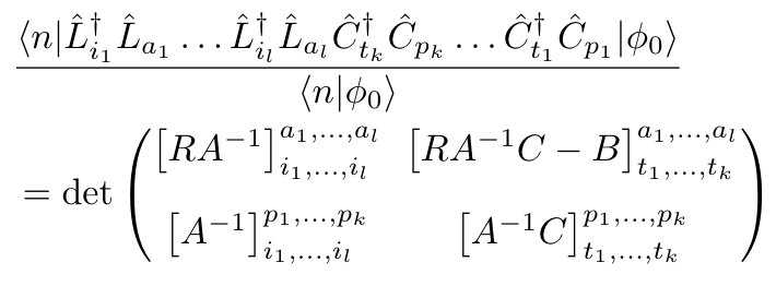
general formula

Using intermediates to speed up sums

With these Green's functions, local energy can be calculated at cost $O(N^4N_c)$ , which is still very expensive when $N_c > 10^3$ .

There's a pattern in the contribution of a configuration to the local energy:

\dfrac{\langle n|\hat{H}_2|\phi_i\rangle}{\langle n|\phi_0\rangle} =

\dfrac{\langle n|\hat{H}_2|\phi_i\rangle}{\langle n|\phi_0\rangle} =

the bottom right block of the determinants is the same

Using this observation, local energy calculation can be performed at cost $O(N^5+N_c)$ , by storing some intermediates.

(This concept is analogous to when performing the product of three matrices $A\times B\times C$ , one stores $A\times B$ or $B\times C$ as an intermediate)

Polyacetylene calculations

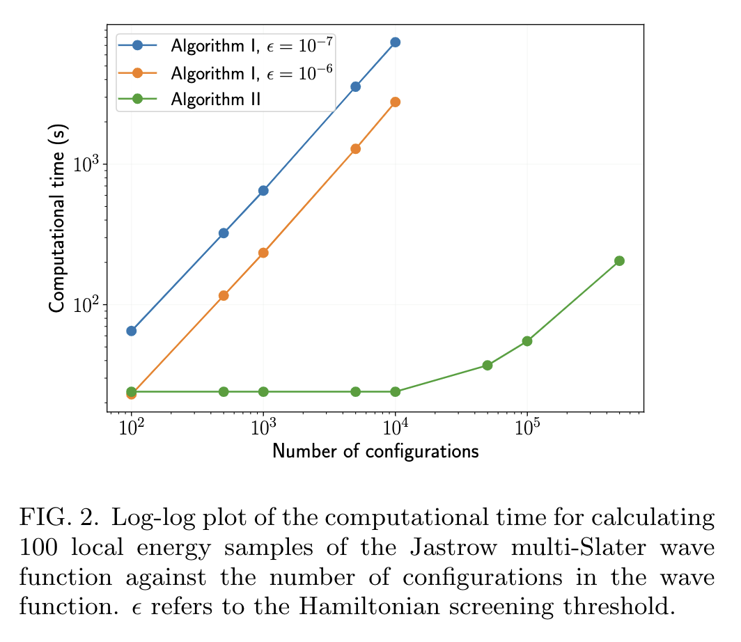
$n = 28$ : active space of $\pi$ orbitals (28e, 28o)

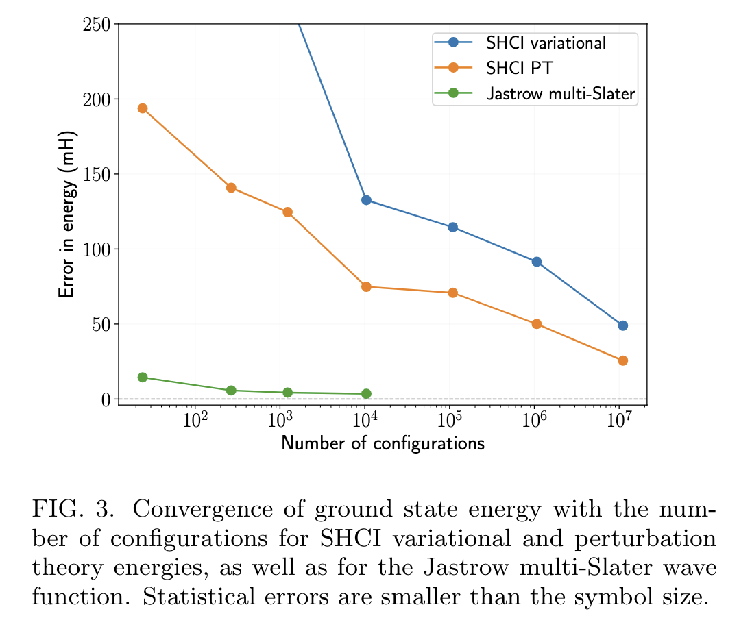
arXiv:2008.06477

Challenges

Dynamic correlation: effect of non-valence virtual orbitals. Important for quantitative accuracy

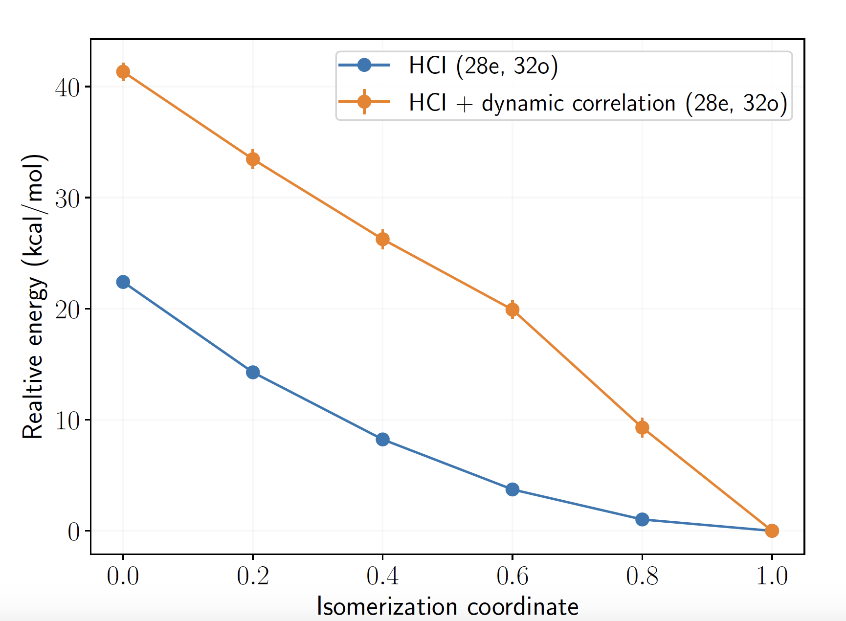
[ $\text{Cu}_2\text{O}_2$ ]

arXiv:2008.00220

VMC optimization limits the number of configurations that can be feasibly used

Both of these could be potentially tackled by using projection Monte Carlo

Auxiliary field quantum Monte Carlo

Imaginary time evolution (projection)

\hat{H} = \sum h_{ia}\hat{c}_a^{\dagger}\hat{c}_{i}+\sum v_{ijab}\hat{c}^{\dagger}_a\hat{c}_b^{\dagger}\hat{c}_j\hat{c}_i,

\hat{H} = \sum h_{ia}\hat{c}_a^{\dagger}\hat{c}_{i}+\sum v_{ijab}\hat{c}^{\dagger}_a\hat{c}_b^{\dagger}\hat{c}_j\hat{c}_i,

Exponential of one body part can be calculated in $O(N^3)$ time, but that of the two-body part very expensive to do exactly.

Approximations:

Hartree-Fock or DFT: replace operator terms with scalar mean values

\hat{c}_a^{\dagger}\hat{c}_b^{\dagger}\hat{c}_j\hat{c}_i\rightarrow \hat{c}_a^{\dagger}\hat{c}_i\langle\hat{c}_b^{\dagger}\hat{c}_j\rangle-\hat{c}_a^{\dagger}\hat{c}_j\langle\hat{c}_b^{\dagger}\hat{c}_i\rangle

\hat{c}_a^{\dagger}\hat{c}_b^{\dagger}\hat{c}_j\hat{c}_i\rightarrow \hat{c}_a^{\dagger}\hat{c}_i\langle\hat{c}_b^{\dagger}\hat{c}_j\rangle-\hat{c}_a^{\dagger}\hat{c}_j\langle\hat{c}_b^{\dagger}\hat{c}_i\rangle

AFQMC: Perform Hubbard Stratanovic transform and sample boson fields

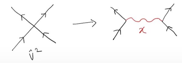
e^{-\frac{\tau}{2}\hat{v}^2}=\int\frac{dx}{\sqrt{2\pi}}e^{-\frac{x^2}{2}+i\sqrt{\tau}x\hat{v}}

e^{-\frac{\tau}{2}\hat{v}^2}=\int\frac{dx}{\sqrt{2\pi}}e^{-\frac{x^2}{2}+i\sqrt{\tau}x\hat{v}}

Sign problem $\rightarrow$ trial function $\rightarrow$ multi-Slater

$\exp(-\tau\hat{H})|\phi\rangle \rightarrow$ ground state, for $\tau\rightarrow\infty$

Jastrow multi-Slater electronic wave functions

Challenging electronic structure problems

Local and canonical descriptions

Local and canonical descriptions

Variational principle

Local energy of Jastrow multi-Slater

Overlaps are determinants

Generalized Wick's theorem

Using intermediates to speed up sums

Polyacetylene calculations

Challenges

Auxiliary field quantum Monte Carlo

Thank you!