Why study dynamics?

Directly related to experiments: electronic response to experimental probes

At finite temperatures, electron dynamics are always present

Goal: Develop a set of ab initio methods to study electron dynamics in strongly correlated molecular and condensed systems

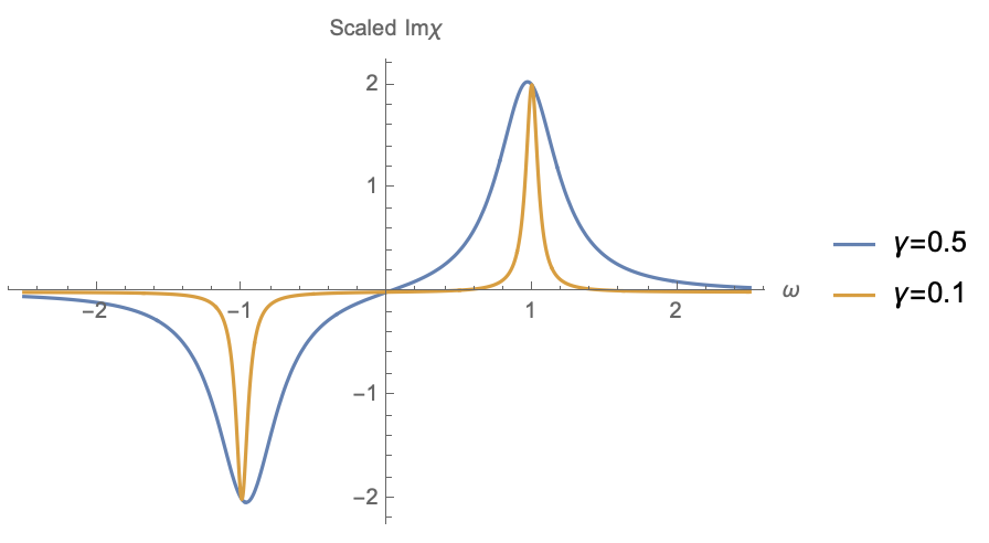
Damped harmonic oscillator

\ddot{x}+\gamma\dot{x}+\omega_o^2x =F(t)

\ddot{x}+\gamma\dot{x}+\omega_o^2x =F(t)

Response to an external time-dependent force $F(t)$

x(t) = \int_{-\infty}^{\infty} dt' \chi(t-t')F(t') \xrightarrow{\mathcal{F}} x(\omega) = \chi(\omega) F(\omega)

x(t) = \int_{-\infty}^{\infty} dt' \chi(t-t')F(t') \xrightarrow{\mathcal{F}} x(\omega) = \chi(\omega) F(\omega)

\chi(\omega) = \dfrac{1}{-\omega^2+i\gamma\omega+\omega_0^2}

\chi(\omega) = \dfrac{1}{-\omega^2+i\gamma\omega+\omega_0^2}

green's function, susceptibility, response function, ...

\chi(\tau)\propto\Theta(\tau)e^{-\gamma\tau/2}

\chi(\tau)\propto\Theta(\tau)e^{-\gamma\tau/2}

\text{Im}\chi(\omega) = \dfrac{\omega\gamma}{(\omega_0^2-\omega^2)^2+\gamma^2\omega^2}

\text{Im}\chi(\omega) = \dfrac{\omega\gamma}{(\omega_0^2-\omega^2)^2+\gamma^2\omega^2}

Spectral function $\propto$ dissipation ( $\gamma$ )

\omega_{\pm}=-\dfrac{i\gamma}{2}\pm\sqrt{\omega_0^2-\gamma^2/4}

\omega_{\pm}=-\dfrac{i\gamma}{2}\pm\sqrt{\omega_0^2-\gamma^2/4}

Poles:

Linear response functions in QM

Suppose a system is perturbed as $H_{ext} = F(t)\hat{B}$ , then the response of $\langle\hat{A}\rangle$ to linear order is given by

\delta\langle\hat{A}\rangle(t) = \int_{-\infty}^{\infty}\chi_{AB}(t-t')F(t')dt'

\delta\langle\hat{A}\rangle(t) = \int_{-\infty}^{\infty}\chi_{AB}(t-t')F(t')dt'

Kubo formula:

\chi_{AB}(t-t') =-i\Theta(t-t')\langle[\hat{A}(t),\hat{B}(t')]\rangle_0

\chi_{AB}(t-t') =-i\Theta(t-t')\langle[\hat{A}(t),\hat{B}(t')]\rangle_0

Spectral representation:

\chi_{AB}(\omega) = \sum_{m\neq0}\dfrac{\langle\psi_0|\hat{A}|\psi_m\rangle\langle\psi_m|\hat{B}|\psi_0\rangle}{\omega-(E_m-E_0)+i\eta} - \dfrac{\langle\psi_0|\hat{B}|\psi_m\rangle\langle\psi_m|\hat{A}|\psi_0\rangle}{\omega-(E_0-E_m)+i\eta}

\chi_{AB}(\omega) = \sum_{m\neq0}\dfrac{\langle\psi_0|\hat{A}|\psi_m\rangle\langle\psi_m|\hat{B}|\psi_0\rangle}{\omega-(E_m-E_0)+i\eta} - \dfrac{\langle\psi_0|\hat{B}|\psi_m\rangle\langle\psi_m|\hat{A}|\psi_0\rangle}{\omega-(E_0-E_m)+i\eta}

For the case $\hat{A} = \hat{B}$ , dissipation $\propto$ fluctuations

\text{Im}\chi(\omega)=-\pi\sum_{m\neq0}|\langle\psi_0|\hat{A}|\psi_m\rangle|^2\delta(\omega-(E_n-E_0))\propto\langle \hat{A}(\omega)\hat{A}(0)\rangle_0

\text{Im}\chi(\omega)=-\pi\sum_{m\neq0}|\langle\psi_0|\hat{A}|\psi_m\rangle|^2\delta(\omega-(E_n-E_0))\propto\langle \hat{A}(\omega)\hat{A}(0)\rangle_0

Fermi's golden rule: scattering amplitude for probe particle, could be a photon, neutron, electron, etc.

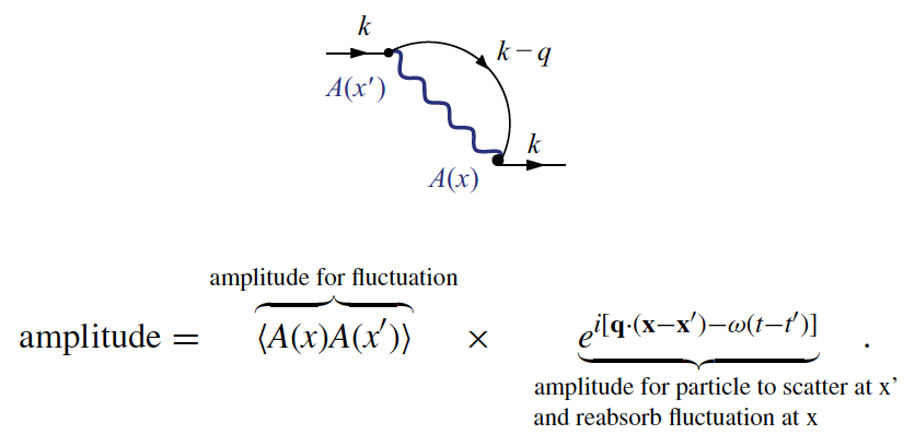
Different spectroscopies couple to different operators $\hat{A}$

Photoemission/attachment: $\hat{c}_{\mathbf{k}}$ , $\hat{c}_{\mathbf{k}}^{\dagger}$

X-ray scattering: $\rho(x)$

neutorn scattering: $\rho_{\sigma}(x)$

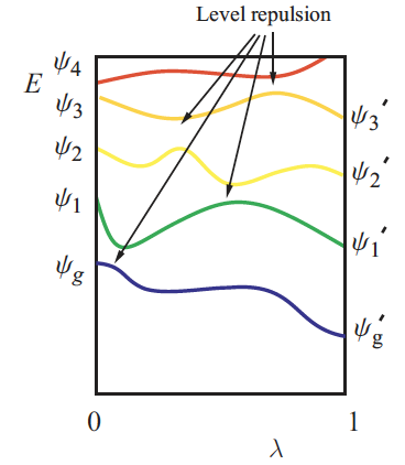
Adiabatic theorem: Elementary excitations of the electron Fermi liquid

Model condensed system: interacting electron liquid, compensating uniform background

In the noninteracting limit, reduces to free Fermi gas with excitations described by free electrons and holes

Adiabatic theorem: If you imagine turning on the interaction slowly, these simple states evolve into quasiparticles

How can we describe particle-hole excitations?

Add excitations to interacting ground-state:

|\psi_{\mathbf{q}}\rangle=c_{\mathbf{k}+\mathbf{q}}^{\dagger}c_{\mathbf{k}}|\psi_0\rangle

|\psi_{\mathbf{q}}\rangle=c_{\mathbf{k}+\mathbf{q}}^{\dagger}c_{\mathbf{k}}|\psi_0\rangle

Construct effective Hamiltonian for these states that encodes interactions between them

H^{\text{eff}}_{\mathbf{q}\mathbf{q'}}=\langle\psi_{\mathbf{q}}|H|\psi_{\mathbf{q'}}\rangle

H^{\text{eff}}_{\mathbf{q}\mathbf{q'}}=\langle\psi_{\mathbf{q}}|H|\psi_{\mathbf{q'}}\rangle

Find low-lying eigenvalues of this effective Hamiltonian to find excitation energies

This approach is very general and used in traditional theories like equation of motion CCSD

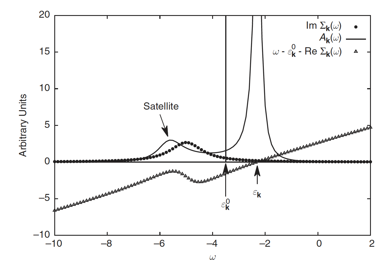
Strong interactions destroy quasiparticles

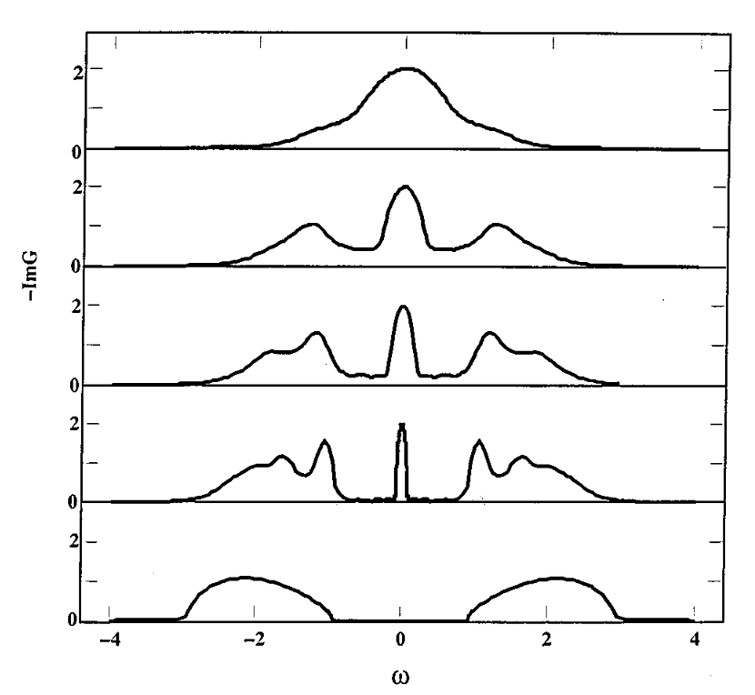
Hubbard model: undergoes Mott transition at critical $U$ , even at zero temperature!

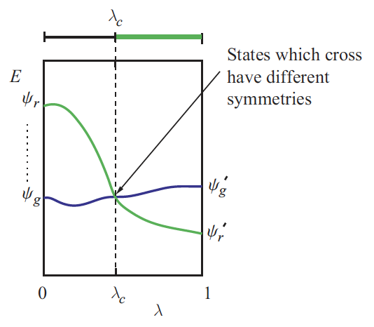
H = \sum_{\langle ij\rangle,\sigma}(c_{i\sigma}^{\dagger}c_{j\sigma}+\text{h.c.}) +\sum_{i}Un_{i\uparrow}n_{j\downarrow}

H = \sum_{\langle ij\rangle,\sigma}(c_{i\sigma}^{\dagger}c_{j\sigma}+\text{h.c.}) +\sum_{i}Un_{i\uparrow}n_{j\downarrow}

For small $U$ , behaves like a weakly interacting Fermi liquid

As $U$ is increased, electrons become localized and the system becomes an insulator, no explanation in terms of quasiparticles possible

Describing correlated excitations

Same strategy as before, act excitations onto the ground state, now in terms of local orbitals

|\psi_{ij}\rangle=a_{i}^{\dagger}a_{j}|\psi_0\rangle

|\psi_{ij}\rangle=a_{i}^{\dagger}a_{j}|\psi_0\rangle

Construct an effective Hamiltonian for these states and find low lying states

Numerically, deterministic algorithms require construction of high-rank reduced density matrices to accomplish this

|\psi_0\rangle=\hat{\mathcal{J}}\hat{P}|\phi\rangle

|\psi_0\rangle=\hat{\mathcal{J}}\hat{P}|\phi\rangle

We use Jastrow symmetry projected mean field states

A way to avoid RDM's: use stochastic sampling

\dfrac{\langle\psi_{\mu}|H|\psi_{\nu}\rangle}{\langle{\psi_s}|{\psi_s}\rangle} = \sum_n\dfrac{|\langle n|\psi_s\rangle|^2}{\langle\psi_s|\psi_s\rangle}\dfrac{\langle\psi_{\mu}|n\rangle}{\langle\psi_{s}|n\rangle}\dfrac{\langle n|H|\psi_{\nu}\rangle}{\langle n|\psi_s\rangle}

\dfrac{\langle\psi_{\mu}|H|\psi_{\nu}\rangle}{\langle{\psi_s}|{\psi_s}\rangle} = \sum_n\dfrac{|\langle n|\psi_s\rangle|^2}{\langle\psi_s|\psi_s\rangle}\dfrac{\langle\psi_{\mu}|n\rangle}{\langle\psi_{s}|n\rangle}\dfrac{\langle n|H|\psi_{\nu}\rangle}{\langle n|\psi_s\rangle}

walker

Generate Hamiltonian excitations from the walker using heat-bath screened sampling

We implemented this for multireference configuration interaction calculations which require similar Hamiltonian construction

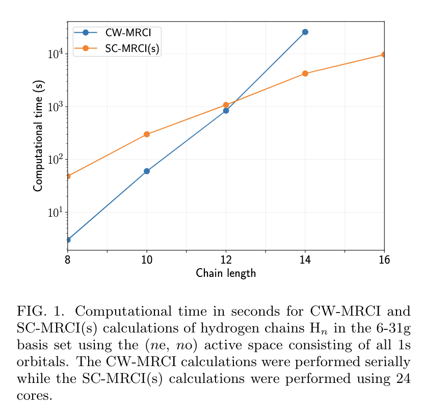
Preliminary results for excited states

Improvements: need to include more excitation classes, e.g. cofermions

Hydrogen chain of 10 atoms, near equilibrium geometry

z_{i\sigma}=c_{i\sigma}n_{i\bar{\sigma}}

z_{i\sigma}=c_{i\sigma}n_{i\bar{\sigma}}

Time-dependent variational principle

A variational principle for the time-dependent Schrodinger equation!

\langle\delta\psi|\left(H-i\partial_t\right)|\psi\rangle = 0

\langle\delta\psi|\left(H-i\partial_t\right)|\psi\rangle = 0

Geometrically:

Expand wavefunction linearly in parameters at $|\psi_0\rangle$ , and diagonalize the effective Hamiltonian in the tangent space:

Another approach to get excited states

Numerically, all gradients can be evaluated at the same cost as the function!

Variational description of electron dynamics