Blockchain 2: Decentralized Crypto-Trading 2023

Traditional Markets

What is Market Microstructure?

How do trading institutions affect market outcomes, e.g.
- trading costs
- information efficiency
- allocative efficiency
A lot of tricky issues
- no one model can do it all
- complex theoretical problems (e.g., infinite regress)
- large datasets

Broker

Exchange

Internalizer

Wholeseller

Darkpool

Venue

Settlement

Traditional Institutions

Investors

Trading Arrangements

central limit order book

complexity

impact of trades

anonymity

price discovery

centralized auction

bilateral
negotiation

Request
for Quote

open
outcry

marginal pricing function

quantity $Q$

price $p(Q)$

Illustration of pricing

quantity

price

$Q$

$p(Q)$

$P^{\mathsf{up}}(Q)=p(Q)\times Q$

Illustration of pricing: auctions/open outcry/RFQ: uniform price

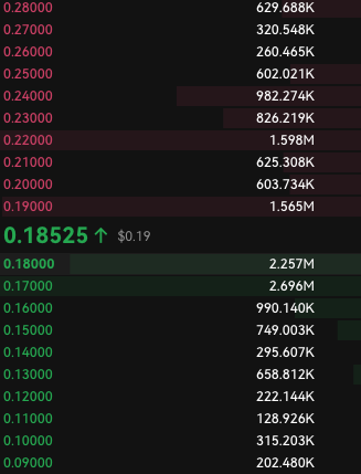
Illustration of pricing: limit order book = discriminatory pricing

quantity

price

$Q$

$p(Q)$

$P^{\mathsf{dp}}(Q)=\int_0^Qp(q)~dq$

Who trades?

Most of the time there is no "coincidence of wants"
$\Rightarrow$ Need liquidity providers!

What's there first?
- trader's order $\equiv$ liquidity provision
- trader's order $\to$ liquidity provision
- liquidity provision $\to$ trader's orders
Deeply affects models and modelling choices

Key question for liquidity provision

Why is there trading?
- diversification/liquidity shocks
- private information

Seminal papers

trader's order $\equiv$ liquidity provision
- Grossman & Stiglitz (AER 1980)
trader's order $\to$ liquidity provision
- Kyle (ECTA 1985)
- Grossman & Miller (JF 1988)
liquidity provision $\to$ trader's orders
- Glosten & Milgrom (JFE 1986)
- Foucault (JFM 1999)

What's there first? Orders or Liquidity?

Seminal papers

trader's order $\equiv$ liquidity provision
- Grossman & Stiglitz (AER 1980)
trader's order $\to$ liquidity provision
- Kyle (ECTA 1985)
- Grossman & Miller (JF 1988)
liquidity provision $\to$ trader's orders
- Glosten & Milgrom (JFE 1986)
- Foucault (JFM 1999)

people "buy" noisy information
demand = supply
price reveals information
marginal value of info = cost of info

competitive liquidity provider receives order flow and sets zero-profit price
noise trader order flow
monopolist informed trader cautiously trades over time to conceal info
slope of the price curve measures liquidity

risk-averse market makers require compensation for risk-taking (position risk)
liquidity-motivated traders submits order
what determines the price slope?

informed and uninformed arrive in random sequence at the market
market maker posts bid and ask prices that account for info-driven loss
what determines the spread?

submit market vs limit order?
post limit order = trading option for others
fundamental may change and may not be able to adjust limit order
gives rise to price slope and spread

Basics of liquidity provision under value uncertainty

fundamental value up
- $\Rightarrow$ price up
  - $\Rightarrow$ sell the asset for less than its worth
fundamental value down
- $\Rightarrow$ price up
  - $\Rightarrow$ buy the asset for more than its worth

Questions:

Are there fees/cash sources of income?
When does/did the value change?
When do I assess the positional gain/loss?

liquidity provision = accept a risk
risk = fundamental value may change (or may have already changed and you don't know it)

every model has some form of structure like

\[\text{trading fee income} +\underbrace{\text{what I sold it for}-\text{value of net position}}_{\text{positional gain/loss}} \ge 0 \]

Example 1: Grossman/Miller

Any position is a risk $\to$ cost
always over-price the trade to compensate for risk

Example 2: Kyle or Glosten-Milgrom

trade with informed:
- receive too little/pay too much
trade with uninformed:
- pay too little/receive too much
trade-by-trade view
- can either trade on "other" market
- hold asset to maturity

Example 3: Limit order market (a la Glosten 1994)

trade with uninformed:
- overprice small orders
trade with informed:
- underprice small orders

Small point:

Regret free prices: after you see the trade, you don't want to change the price
Kyle prices are regret free
Limit order book prices are not regret free: large orders are more informed so you undercharge when a larger order trades against lower priced orders

Crypto Markets

Trading Infrastructure

payments network

Stock Exchange

Clearing House

custodian

beneficial ownership record

seller

buyer

Broker

Exchange

Internalizer

Wholeseller

Darkpool

Venue

Settlement

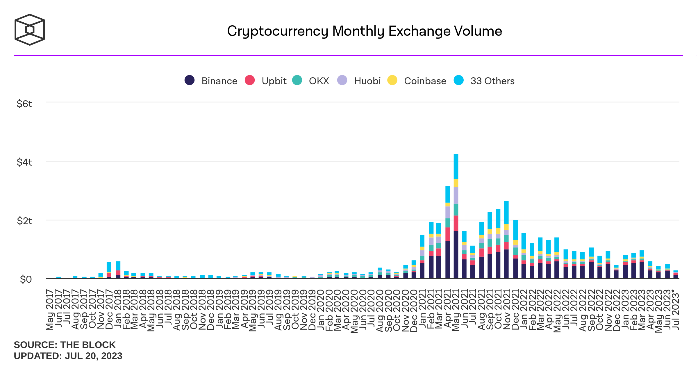
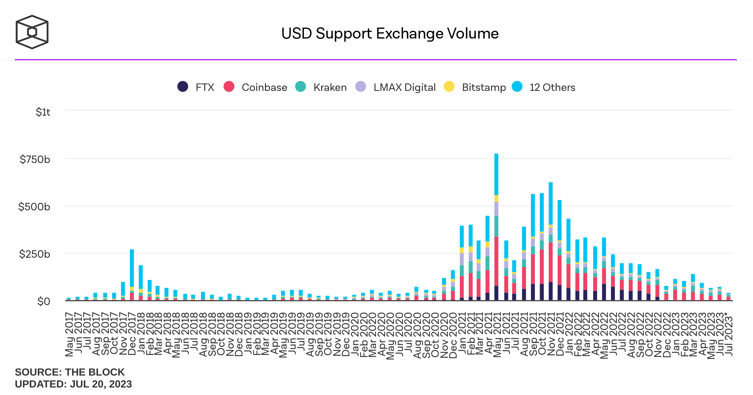
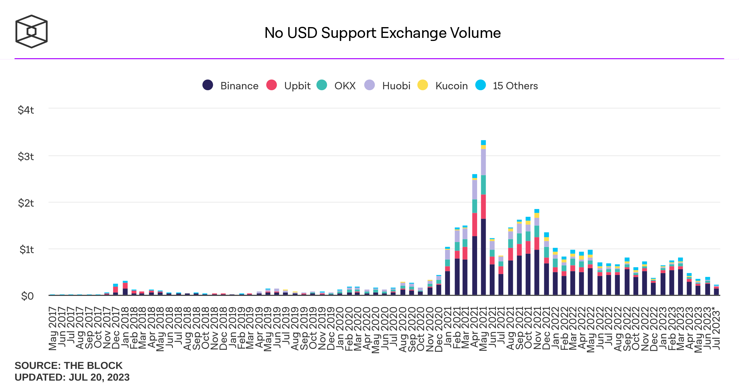
Let's look at some stylized facts

note: Coinbase has only ~260 assets; most trading is in ETH and BTC

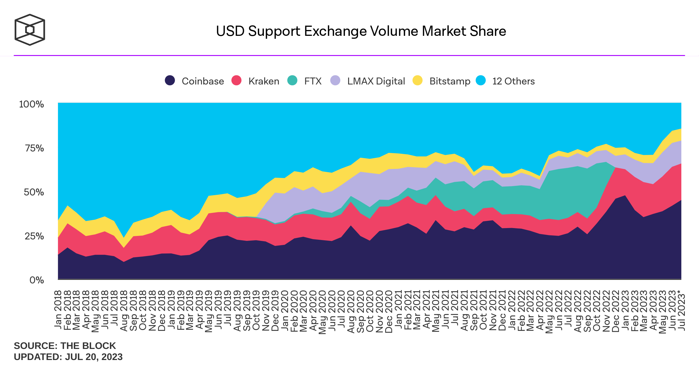
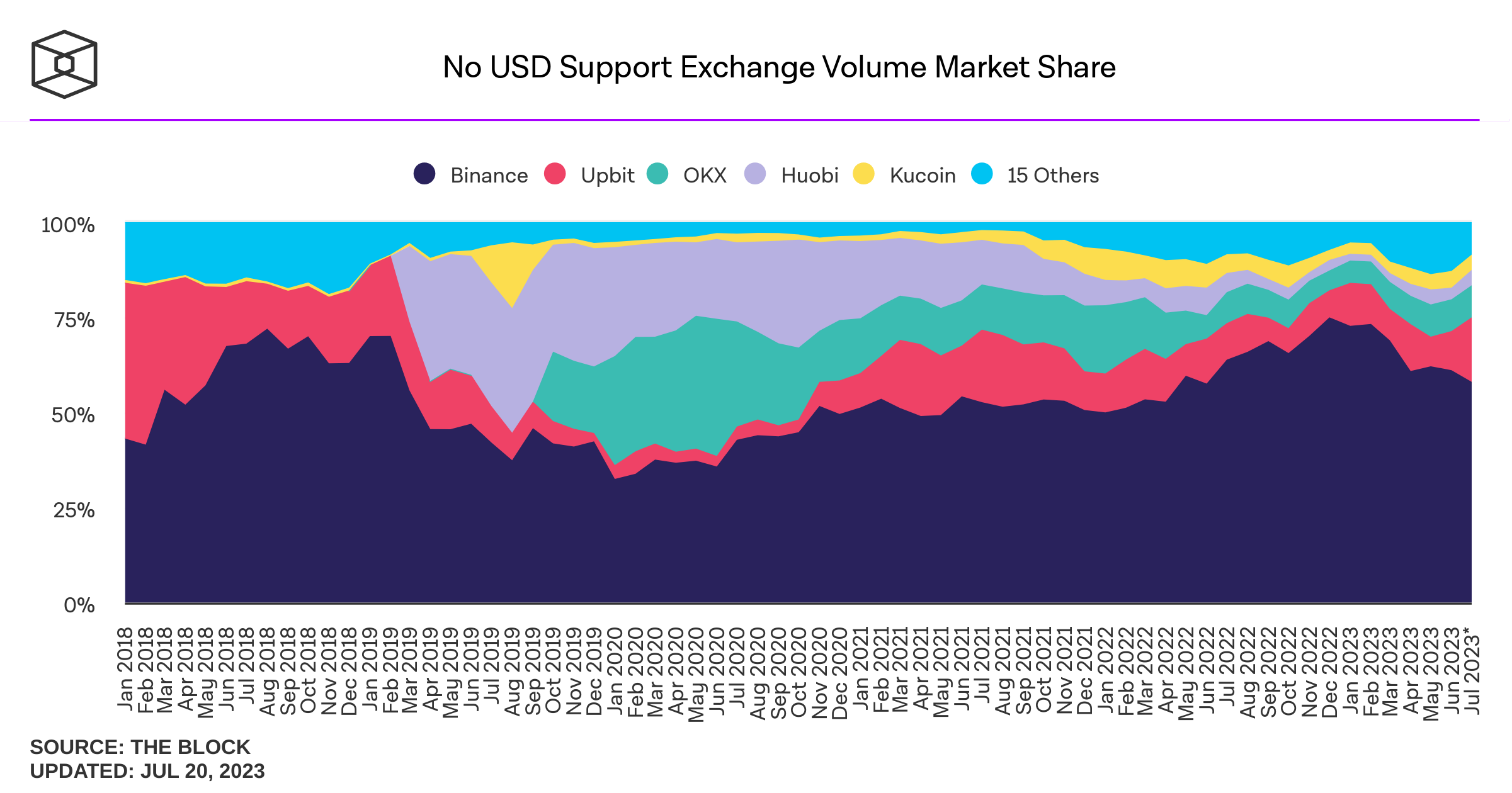
Centralized Trading

Issues and concerns with CEX trading

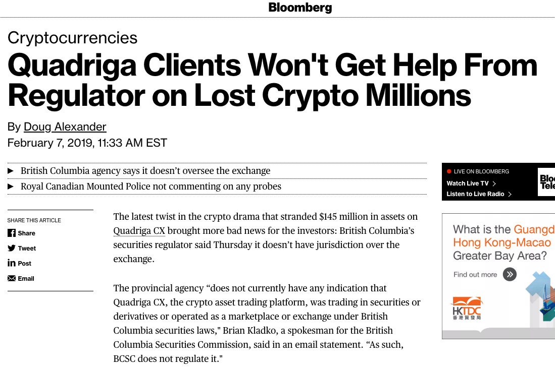
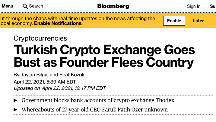
No shortage of drama!
A short list of issues
1. expensive arbitrage
2. price manipulation
3. volume manipulation
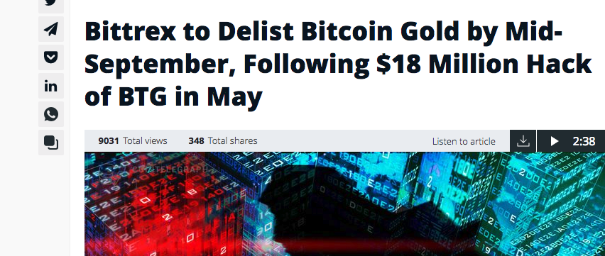
4. security risk
5. Google "Lazarus Group"
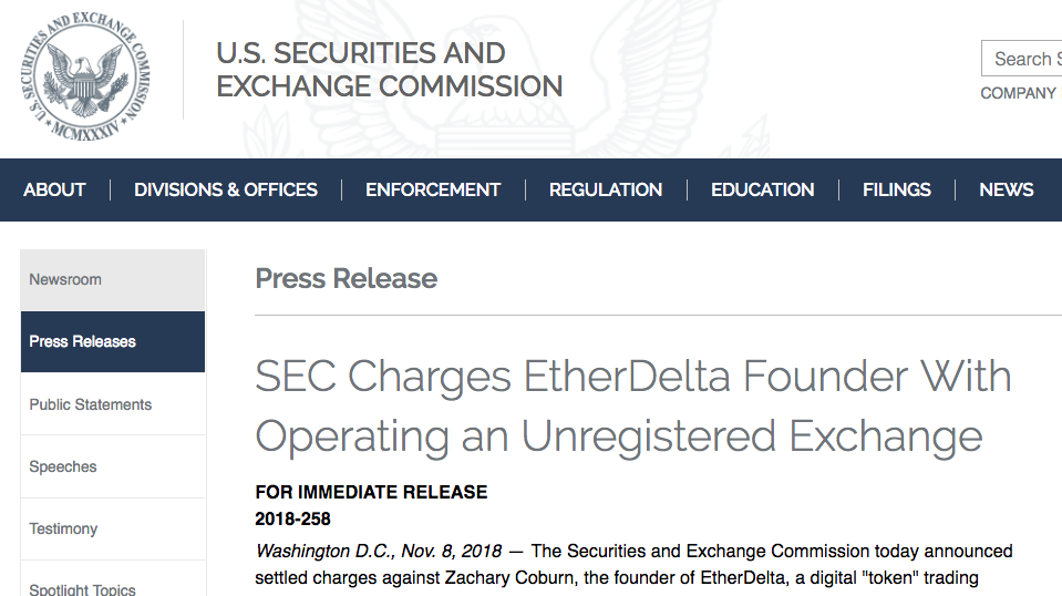
6. Are they unlicensed securities exchanges?

Costly Arbitrage

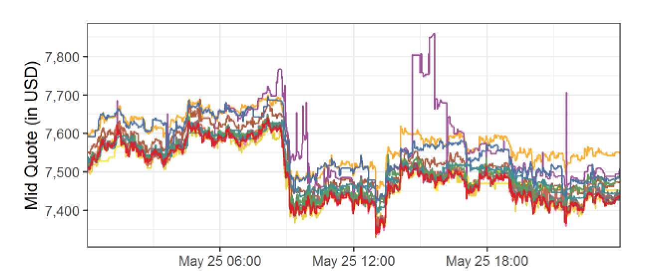
BTC/USD

ask: 7,600

bid: 7,550

BTC/USD

ask: 7,500

bid: 7,450

buy BTC

sell BTC

move BTC to Kraken

=> arbitrage = commit capital on multiple exchanges

Crypto Wash Trading, Lin William Cong, Xi Li, Ke Tang, Yang Yang

systematic tests:
- robust statistical and behavioral patterns in trading to detect fake transactions on 29 cryptocurrency exchanges.
- Regulated exchanges are OK
- unregulated exchanges: rampant manipulations
- wash trading on each unregulated exchange:
  - on average over 70% of the reported volume
  - improve exchange ranking
  - temporarily distort prices

Volume Manipulation

Cryptocurrency Pump-and-Dump Schemes
Tao Li, Donghwa Shin, and Baolian Wang, 2020

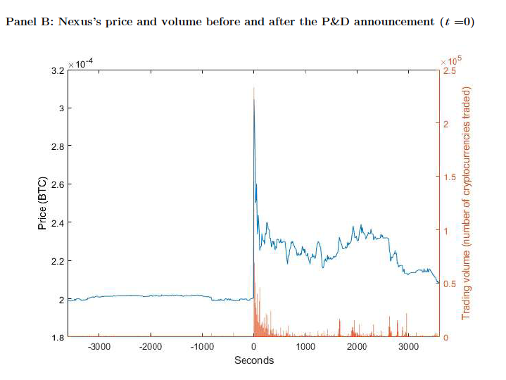
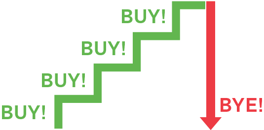
What is pump and dump?

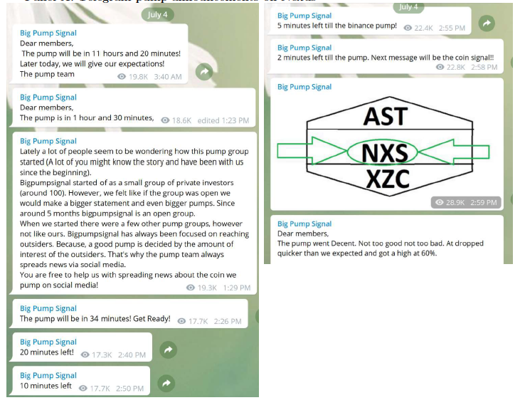
arranged via Telegram Channels

Price Manipulation: Pump & Dump

IS BITCOIN REALLY UN-TETHERED? JOHN M. GRIFFIN and AMIN SHAMS
Journal of Finance 2020

Tether = ‘pushed’
- print an unbacked digital dollar to purchase Bitcoin.
- $\to$ additional supply of Tether creates unwarranted inflation in Bitcoin price

vs.

Tether = ‘pulled’
- driven by legitimate demand from investors who use Tether as a medium of exchange
- $\to$ the price impact of Tether reflects natural market demand

Price Manipulation: Pumping Bitcoin

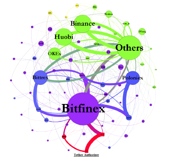
Figure 1. Aggregate Flow of Tether between Major Addresses

August 2016

Security Risk

Decentralized Trading

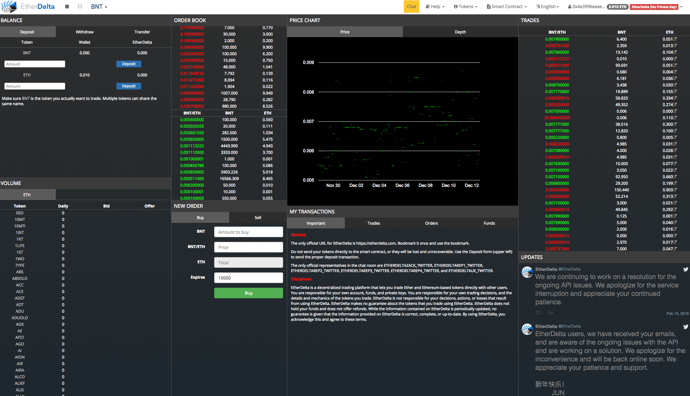
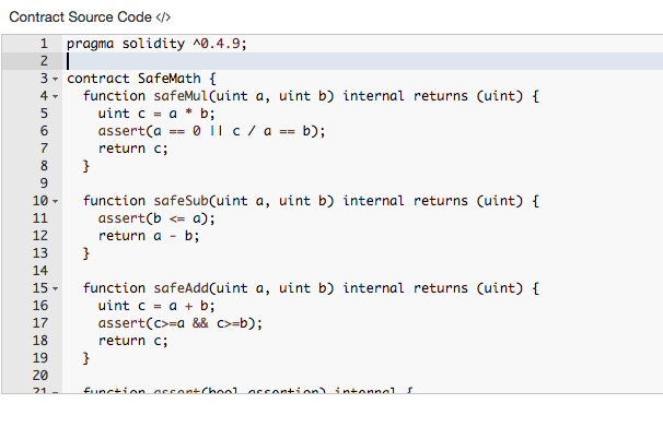
... 300 lines of code ...

Trading Infrastructure

Actually ...

bad idea
Why?
Data-intensive, computation intensive, costly, inefficient

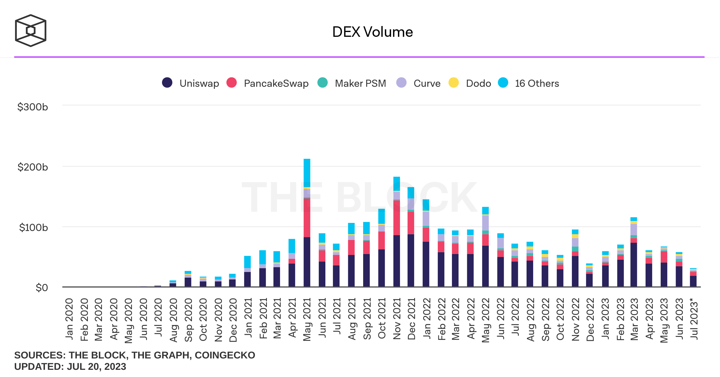
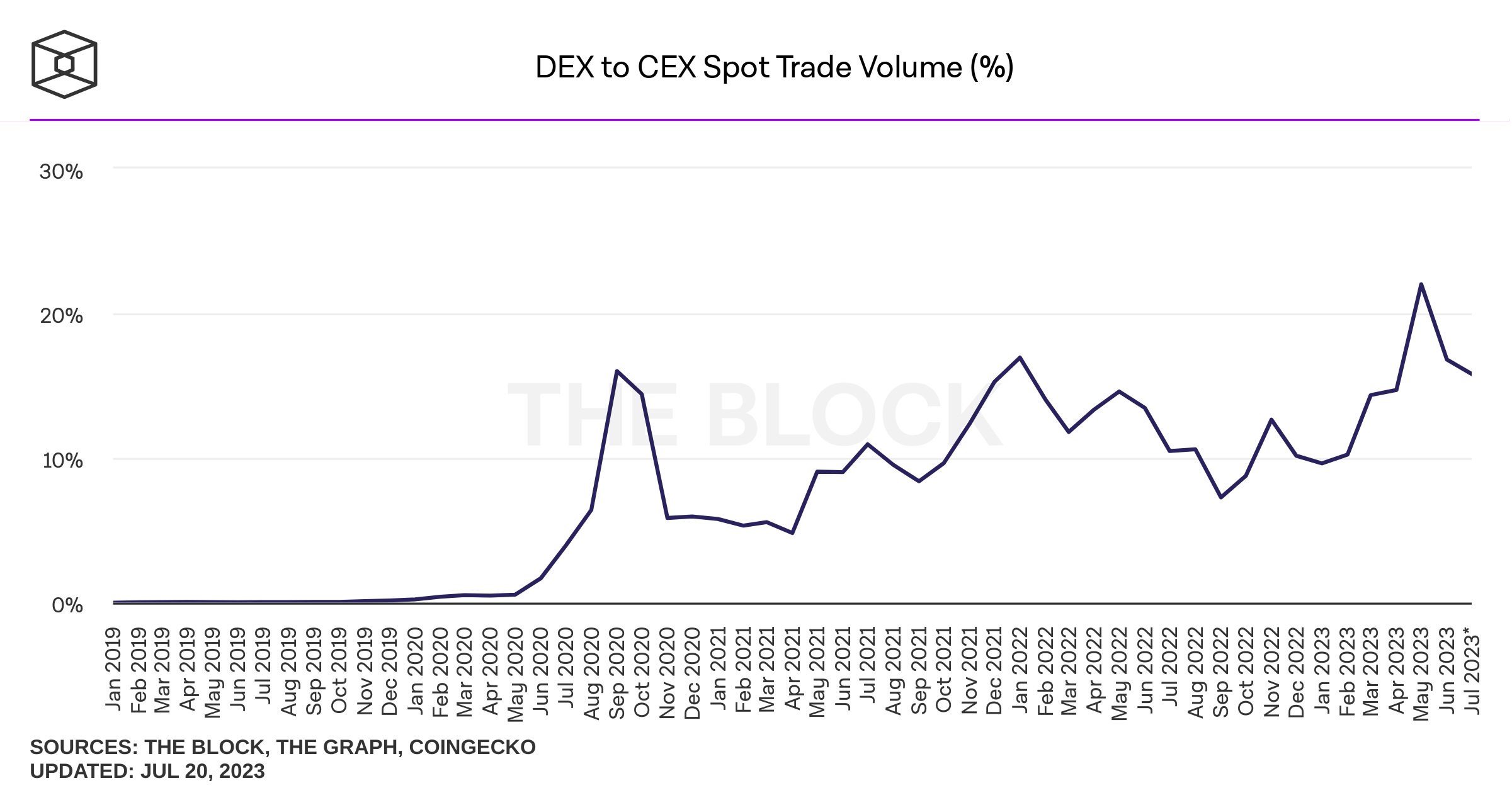
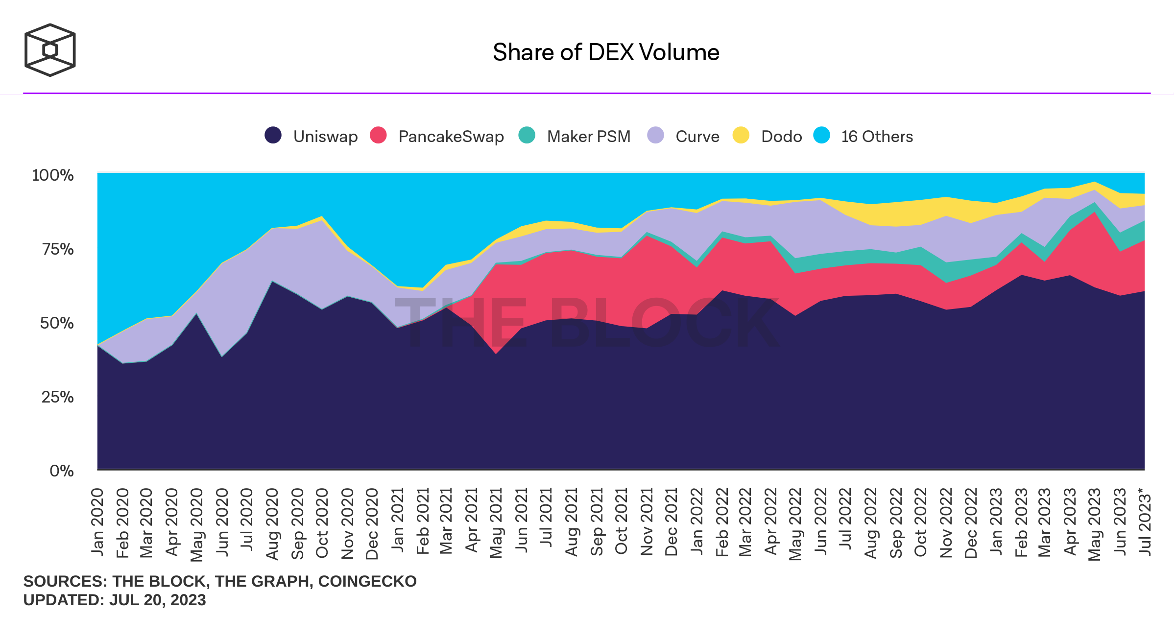
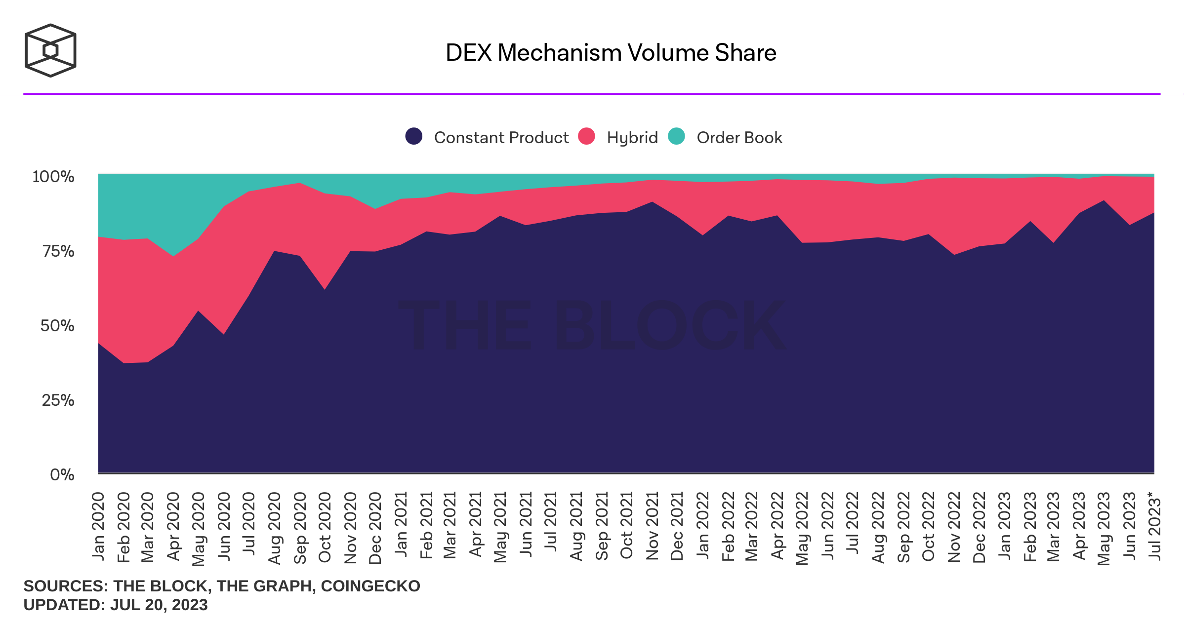
Let's look at some stylized facts

How does it look?

automated market maker

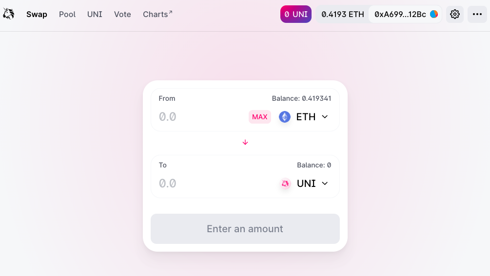
$\to$ simply connect with MetaMask (or similar wallet)

Application: decentralized trading with automated market makers

AMM Pricing

AMMs require liquidity deposits
Deposits:
- $a$ units of an asset (e.g. a stock)
- $c$ units of cash

Constant Liquidity (Product) AMM

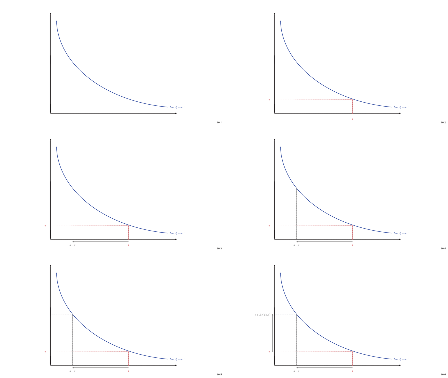
Purchase $q$ of asset
Deposit cash $\Delta c (q)$ into liquidity pool, extract $q$ of shares
Idea of pricing: liquidity before trade $=$ after trade
\[L(a,c)=L(a-q,c+\Delta c)\]

AMMs require liquidity deposits
Deposits:
- $a$ units of an asset (e.g. a stock)
- $c$ units of cash

Key Components

pooling of liquidity

pro-rated
- fee income
- risk

Liquidity providers:
- use existing assets to earn passive income

Liquidity demanders:
- predicatable price
- continuous trading
- ample liquidity

The Pricing Function

Liquidity Deposit $\Rightarrow$ slope of the price curve

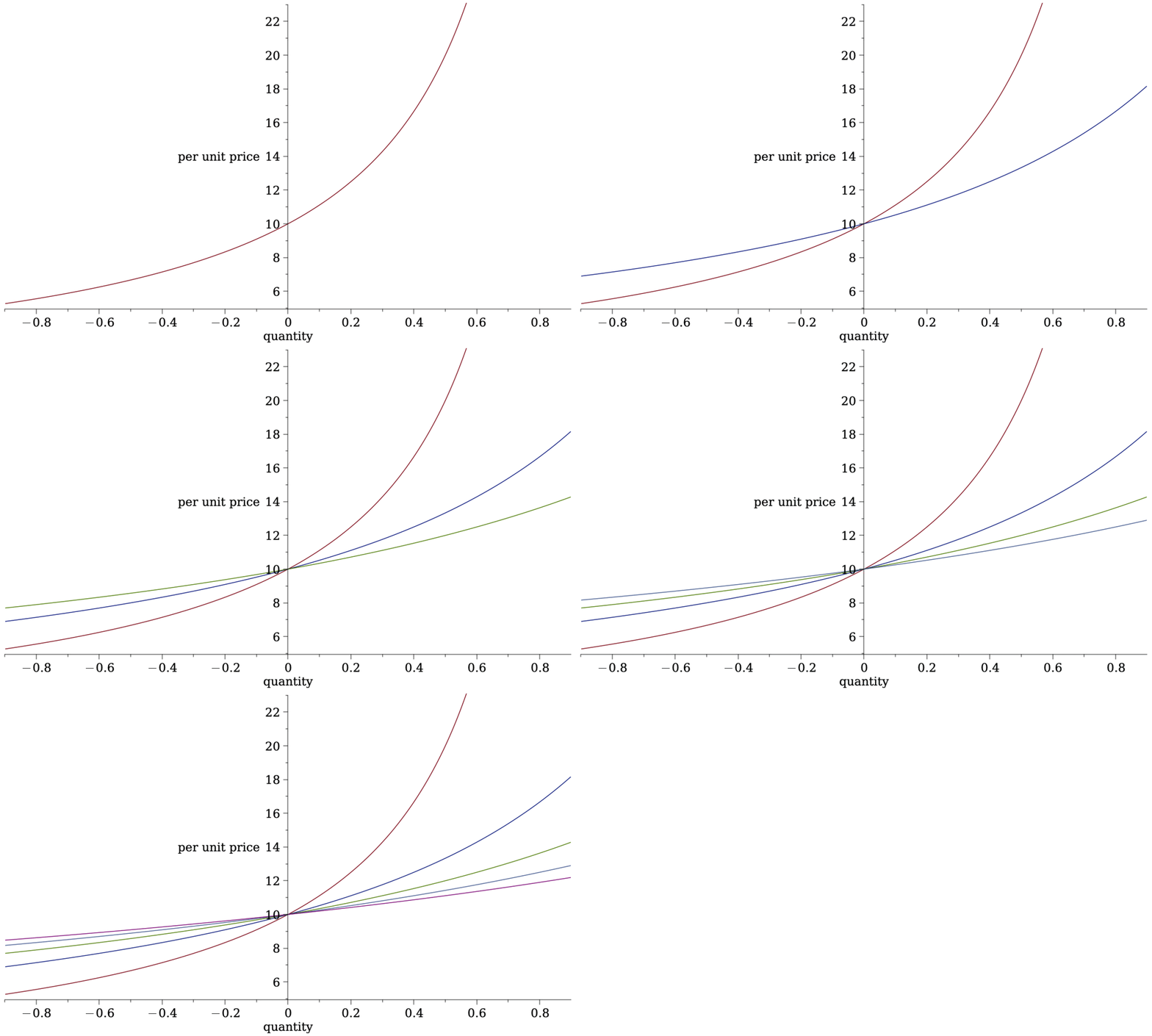
Most common form of AMM liquidity rule is Constant Product Pricing
\[L(a,c)=a\cdot c~\Rightarrow~a\cdot c= (a-q)\cdot (c+\Delta c).\]
Total cost of trading $q$ \[\Delta c=\frac{cq}{a-q}.\]
Price per unit \[p(q)=\frac{c}{a-q}.\]
Average spread paid\[\frac{p(q)}{p(0)}-1=\frac{q}{a-q}.\]

makes asset and cash deposit
more deposits flatter price curve
- attracts more volume
- but larger "positional" loss when prices move

The Pricing Function (just a little more)

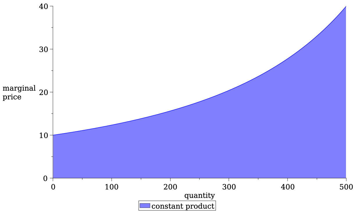
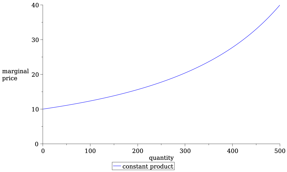
A limit order book has a marginal price function $\rho(q)$ so that \[\Delta c(q)=\int_0^q\rho(s) ds.\]
We can do that here, too: for
\[\rho(q)=\frac{ac}{(a - q)^2},\]
we have \[\int_0^q \frac{ac}{(a - s)^2}ds=\frac{cq}{a-q}.\]
$\to$ Constant Product = special case of a limit order book.

The Pricing Function (just a little more)

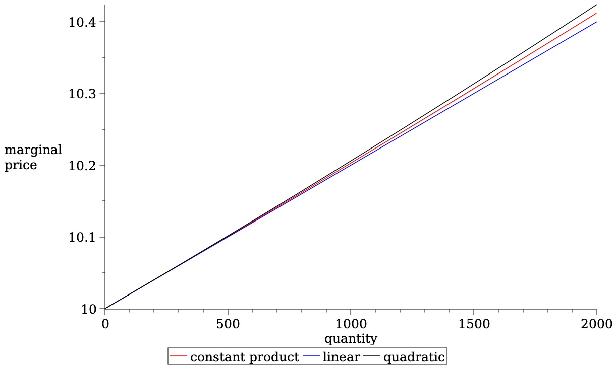
Taylor expansion of $\rho(q)$ around 0?
With $p_0:=c/a$ and get a linear or quadratic approximation:

\begin{array}{rcl} \rho_1(q)&=&p_0+p_0\cdot \frac{2!}{a}\ q ~~\text{or}\\ \rho_2(q)&=&\rho_1(q)+p_0\cdot \frac{3!}{a^2}\ q^2 \end{array}

The Pricing Function (almost done, just one more thing)

Suppose we start with a price $P$ and end with a price $P'=R\cdot P$.

We know by definition
\[P=\frac{c}{a},~P'=\frac{c'}{a'},~L=\sqrt{ac},~L=\sqrt{a'c'}.\]
Then it holds that \[a=\frac{L}{\sqrt{P}},~c=L\sqrt{P},~a'=\frac{L}{\sqrt{P'}},~c'=L\sqrt{P'}.\]

For the price to move from $P$ to $P'$, quantities $q,\Delta c$ change hands.
Therefore $a'=a-q,~c'=c+\Delta c$

Combine with the above \[a-q=\frac{L}{\sqrt{P'}}~\Leftrightarrow~q=L\left(\frac{1}{\sqrt{P}}-\frac{1}{\sqrt{P'}}\right).\]
do the same for $\Delta c$ \[\Delta c= L\left(\sqrt{P'}-\sqrt{P}\right).\]

the per unit price for the trade of $\Delta x$ is \[\frac{\Delta c}{q}=\sqrt{PP'}=P\sqrt{R}.\]
$\to$ avg price is the geometric mean of the prices

AMMs continue to evolve: UniSwap v3

Basic idea:

allow different fees (let's ignore)
don't supply liquidity for entire price range $(0,\infty)$ but only $[p_a,p_b]$

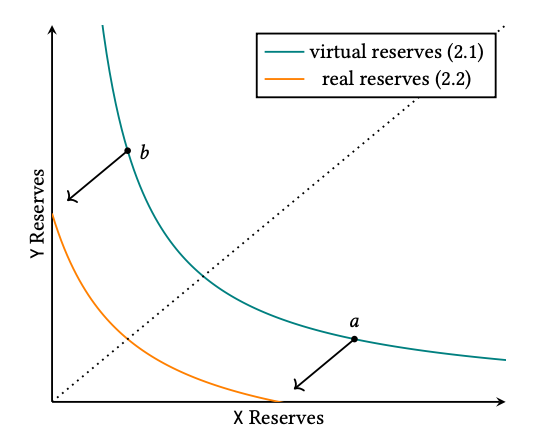
idea: project the iso-liquidity curve back to the axes
price in this range is determined by constant product rule

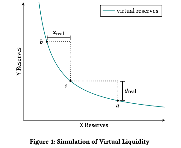
Source:" Uniswap v3 Core," Adams, Zinsmeister, Salem, Keefer, Robinson (2021)

current price at point $c$: $p_c$
$x_{\text{real}}=$ max of $X$ you buy
$y_{\text{real}}=$ max of $Y$ you buy

pricing effectively occurs on a grid
it's not straightforward to describe the pricing function without lots of new notation

More on UniSwap v3

liquidity provision choice in v2:
- submit $a,c$ at the marginal $p_0=\frac{c}{a}$
- $\to$ for given $p_0$, there is ONE degree of freedom
- provide liquidity
  - for all prices $p\in(0,\infty)$
  - all asset amounts $q\in(0,a)$
  - all cash amounts $\Delta c\in (0,c)$

liquidity provision choice in v3:
- submit $u,\Delta c (d)$
- choose price range $[p_d,p_u]$
- provide liquidity
  - for all prices $p\in[p_d,p_u]$
  - all asset amounts $q\in(0,u)$
  - all cash amounts $\Delta c\in (0,\Delta c(d))$
$\to$ for given $p_0$, there are THREE degrees of freedom

More on UniSwap v3

marginal "limit order book" price

\[\gamma(s)=\frac{ac}{(a-s)^2}\]

$p_u=15$

$p_d=7$

$u=2$

$p_0=10$ (that's exogenous, not a choice)

More on UniSwap v3

marginal "limit order book" price

\[\gamma(s)=\frac{ac}{(a-s)^2}\]

$p_u=15$

$p_d=7$

$u=2$

$p_0=10$ (that's exogenous, not a choice)

= find the right curve

= find the right "$a^*$"

More on UniSwap v3

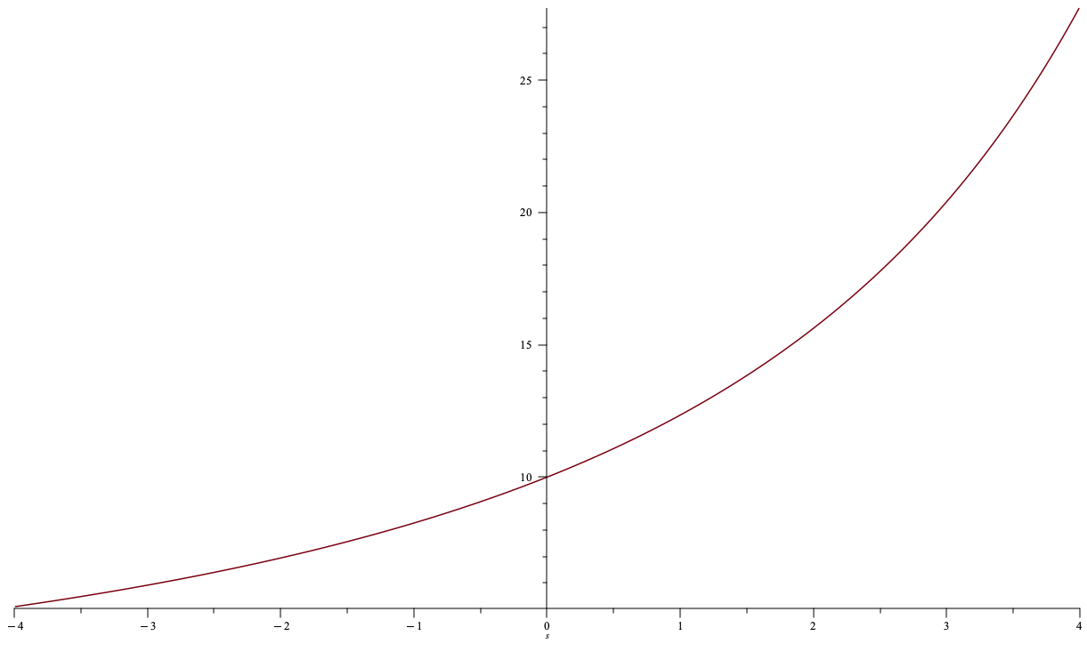
marginal "limit order book" price

\[\gamma(s)=\frac{ac}{(a-s)^2}\]

$p_u=15$

$p_d=7$

$u=2$

$d=?$

required cash deposit $\Delta c(d)=$ the amount that I pay for $d$

Some UniSwap v3 maths (Barbon & Ranaldo 2023)

Source: Elsts (2021) "Liquidity Math in UniSwap v3"

We are interested in "virtual limit orders"
- for selling known $x\Rightarrow y=0$ (only sell) have known $P,x,y,p_a$:
  - what is the (ask) price $p_b$?
- for selling up to price $p_b$ $\Rightarrow y=0$ (only sell) have known $P,y,p_a,p_b$:
  - what is the quantity $x$?

When the price is in interior of $(p_a,p_b)$ liquidity provided "to the left" of the price must coincide with liquidity provided to the right.
We can derive conditions \[x=L\ \frac{\sqrt{p_b}-\sqrt{P}}{\sqrt{p_b}\sqrt{P}}\]
\[y=L\ (\sqrt{P}-\sqrt{p_a})\]

$\tilde{x},\tilde{y}$ the "real" reserves, $x,y$ the virtual reserves
$P$ the price of "$x$" (asset) in "$y$" (cash), with $P\in[p_a,p_b]$
$L$ the liquidity
Constant product function: $L=\sqrt{xy}$
And then \[L^2=\left(\tilde{x}+\frac{L}{\sqrt{p_b}}\right)\left(\tilde{y}+L\sqrt{p_a}\right).\]

At the price bounds, the real amounts are either $x=0$ or $y=0$. We can derive conditions \[x=L\ \frac{\sqrt{p_b}-\sqrt{p_a}}{\sqrt{p_b}\sqrt{p_b}}\]
\[y=L\ (\sqrt{p_b}-\sqrt{p_a})\]

Liquidity Supply and Demand in an Automated Market Maker

Two views

You may trade with uninformed or informed.
- you may have a position gain (against uninformed) or loss (against informed)
- example: Aoyagi and Ito (2021) "Coexisting Exchange Platforms: Limit Order Books and Automated Market Makers", Cartea, Drissi, Monga (2023)
You trade over time with informed and uninformed
- you always lose but get compensated over time
- examples: Lehar and Parlour (2021), Hasbrouck, Riviera, Saleh (2023), Park (2021), Malinova and Park (2023)
- Lehar and Parlour (2021) assume that every uninformed trade is off-set by an arbitrageur $\to$ more fee income

Basics of Liquidity Provision

\[\underbrace{F \int DV \mu(DV) }_{\text{fees earned on}\atop \text{balanced flow}}+\int_0^\infty\underbrace{(\Delta c(q^*)-q^*p_t(R)}_{\text{adverse selection loss} \atop \text{when the return is {\it R}}} +\underbrace{F \cdot \Delta c(q^*))}_{\text{fees earned}\atop \text{from arbitrageurs}}~\phi(R)dR \ge 0.\]

$q^* $ is what arbitrageurs trade to move the price to reflect $R$

Basic idea of liquidity provision: earn more on balanced flow than what you lose on price movement

\[\text{fee income} +\underbrace{\text{what I sold it for}-\text{value of net position}}_{\text{adverse selection loss}} \ge 0 \]

in AMMs:
protocol fee

in tradFi: bid-ask spread

Basics of Liquidity Provision

\[\frac{1}{\text{initial deposit}}\int_0^\infty(\Delta c(q^*)-q^*p_t(R)+F \cdot \Delta c(q^*))~\phi(R)dR +\frac{F p_0 V}{\text{initial deposit}}\ge 0\]

\[\int_0^\infty\left(\frac{\Delta c(q^*)-q^*p_t(R)}{\text{initial deposit}} +F \cdot \frac{\Delta c(q^*)}{\text{initial deposit}}\right)~\phi(R)dR +\frac{F p_0 V}{\text{initial deposit}}\ge 0\]

closed form functions of $R$ only
(see Barbon & Ranaldo (2022))

\[\underbrace{F \int DV \mu(DV) }_{\text{fees earned on}\atop \text{balanced flow}}+\int_0^\infty\underbrace{(\Delta c(q^*)-q^*p_t(R)}_{\text{adverse selection loss} \atop \text{when the return is {\it R}}} +\underbrace{F \cdot \Delta c(q^*))}_{\text{fees earned}\atop \text{from arbitrageurs}}~\phi(R)dR \ge 0.\]

Basics of Liquidity Provision

$\Rightarrow$ $\Delta c(q^*)-q^*p_t(R)$ is also referred to as the "impermanent loss" or "divergence loss"

$\Delta c(q^*)-q^*p_t(R)=\underbrace{p_t(R)\times(a-q^*) +c+\Delta c(q^*)}_{\text{value of liquidity deposit}}-\underbrace{(p_t(R)a+c)}_{\text{value of buy-} \atop \text{and-hold position}}$

see Milionis, Moallemi, Roughgarden, and Zhang (2022) for a dynamic analysis of impermanent loss

Sidebar: we can quantify how much a PASSIVE LP loses when the price moves by $R$

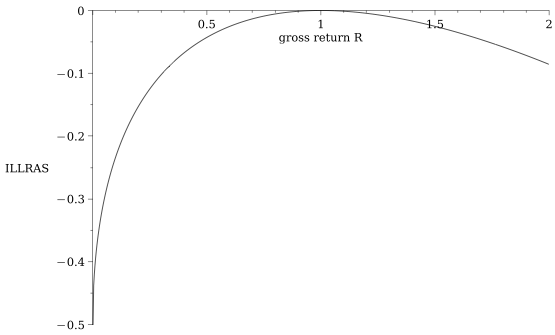
for orientation:

If the stock price drops by 10% the incremental loss for liquidity providers is 13 basis points on their deposit
- $\to$ total loss=-10.13%
If the stock price rises by 10%, the liquidity provider gains 12 basis points less on the deposit
- $\to$ total gain =9.88%

\[\frac{\text{adverse selection loss when the return is $R$}}{\text{initial deposit}}=\sqrt{R}-\frac{1}{2}(R+1)\]

see Barbon & Ranaldo (2022)

Basics of Liquidity Provision

Liquidity provision measured as "collective" deposit $\alpha$ of token's market cap as function of

balanced volume
return distribution
(some authors use explicit functions so they can relate it to asset volatility)
fee

\[E[\text{DL}(R)]+F\cdot E[\text{another function of }R]+F\cdot \frac{\text{E[dollar volume]}}{\text{initial deposit}}\ge 0.\]

\[\text{what I sold it for}-\text{value of net position}+\text{fee income} \ge 0 \]

The Decision of the Liquidity Demander

Wants to trade some quantity $q$ at cost

\[\text{AMM price impact} +\text{AMM fee}.\]

two opposing forces for $F\nearrow$ for liquidity demand
- more liquidity provision
  $\to$ lower price impact
- more fees to pay
Finding: There is a minimal cost fee:

\[F^\pi=\frac{1}{E[|\sqrt{R}-1|/2]+E[DV]}\left(-2q\ E[\text{DL}]+ \sqrt{-2qE[DV]\ E[\text{DL}]}\right).\]

this is from Malinova and Park (2023); similar result is in Hasbrouk, Riviera, Saleh (2023)

Model Summary

Have: equilibrium choice for liquidity provision.
Useful feature: can express liquidity by % market cap of token/asset
Can measure cost for liquidity demanders to use AMM.
Know: fee that maximizes liquidity demander benefit ($\not=0$)

Empirical Work

Lehar and Parlour (2021)

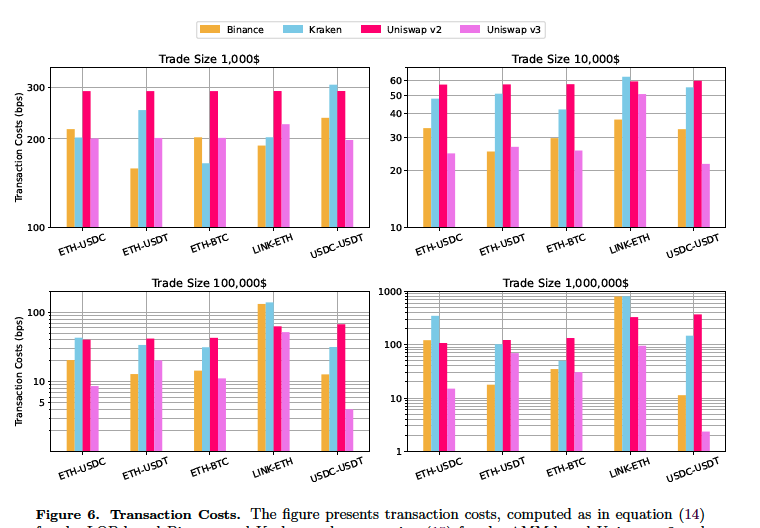
Barbon & Ranaldo (2023)

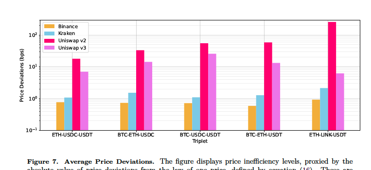
Other notables:

Lehar, Parlour, Zoican (2022):
- study and document fragmentation of liquidity across different fee levels
- most intense provision-withdrawal activity for low fees $\to$ UniSwap v3 starts mimicking tradfi
Capponi & Jia (2022) study impact of curvature of pricing function
- Theory: curvature of optimal pricing curve $\nearrow$ volatility
- Empirics: cost volatility is 60% lower for stable-coin pairs
- corr(deposit inflows ,volatility)<0
  corr(deposit inflows ,volume)>0

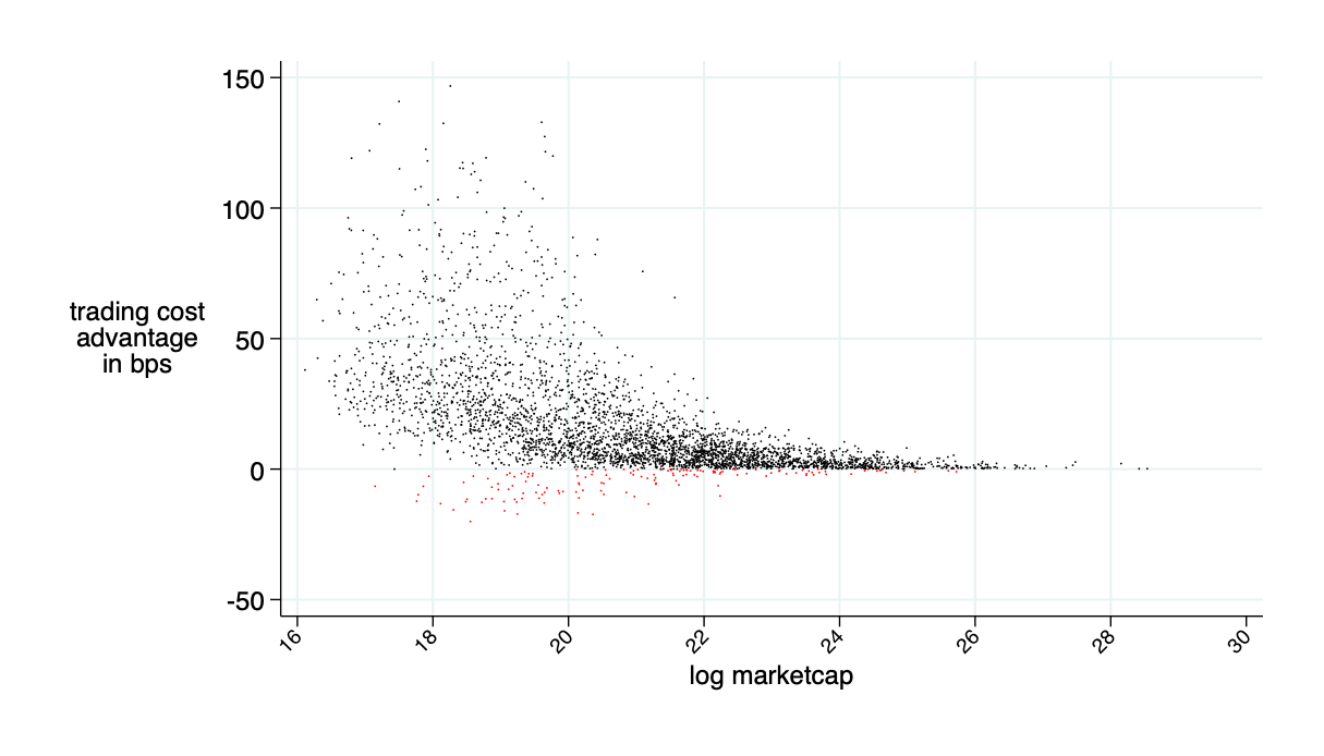
Malinova & Park (2023): AMM applied to equities would reduce trading costs by 30%

Concerns around Automated Market Makers

a

b

c

d

e

f

g

Problem: Public Mempools allow sandwich (MEV) attacks

Problem: MEMPOOL Frontrunning is intrinsically profitable

$X$

$Y$

normal trade: sell $x$ $\to$ get $y'$

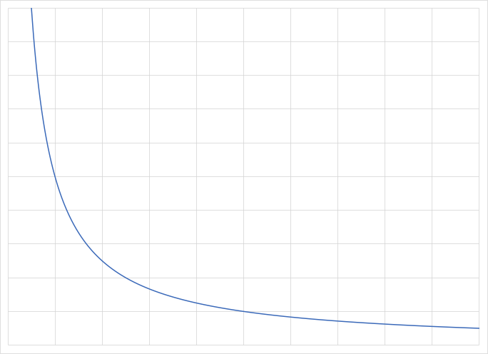
$Y-y'$

$X+x$

front-running:

front-runner: sells $x$ $\to$ gets $y'$
front-run: sells $x$ $\to$ gets $y''$
front-runner: buys $x$ $\to$ pays $y''$

$Y-y'-y''$

$X+2x$

$y'>y''~\Rightarrow$

front-running is intrinsically profitable

Disclaimer:

this problem is well-known
fees can mitigate it
several protocols such as the latest iteration by Balancer try to combat it

From Vitalik Buterin's post on the topic:

https://ethresear.ch/t/improving-front-running-resistance-of-x-y-k-market-makers/1281

February 2022: UniSwap (V2), ETH-USDC
- 38,100 ETH
- 118M USDC
- $p=\$3,097$
Buy: 100 ETH
- pay approximately $3,105 per ETH. accoridng to bonding curve
100 ETH MEV sandwich attack
- Initial trade cost: $3,105 per ETH
- reversing yields $3,121 per ETH
- total profit of $1,639 $=$ value extracted from original trader.
1,000 ETH MEV attack
- profit/loss $=$ $17K
10,000 ETH MEV attack
- profit/loss $=$ $261K.

Theorem (Park 2023):

Constant product pricing and linear limit order book pricing allows unlimited MEV losses
Uniform pricing has limited MEV losses (but other problems)

Hypothetical example

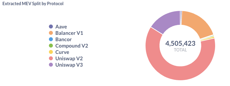
The Bigger Picture: MEV Extraction

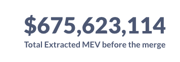
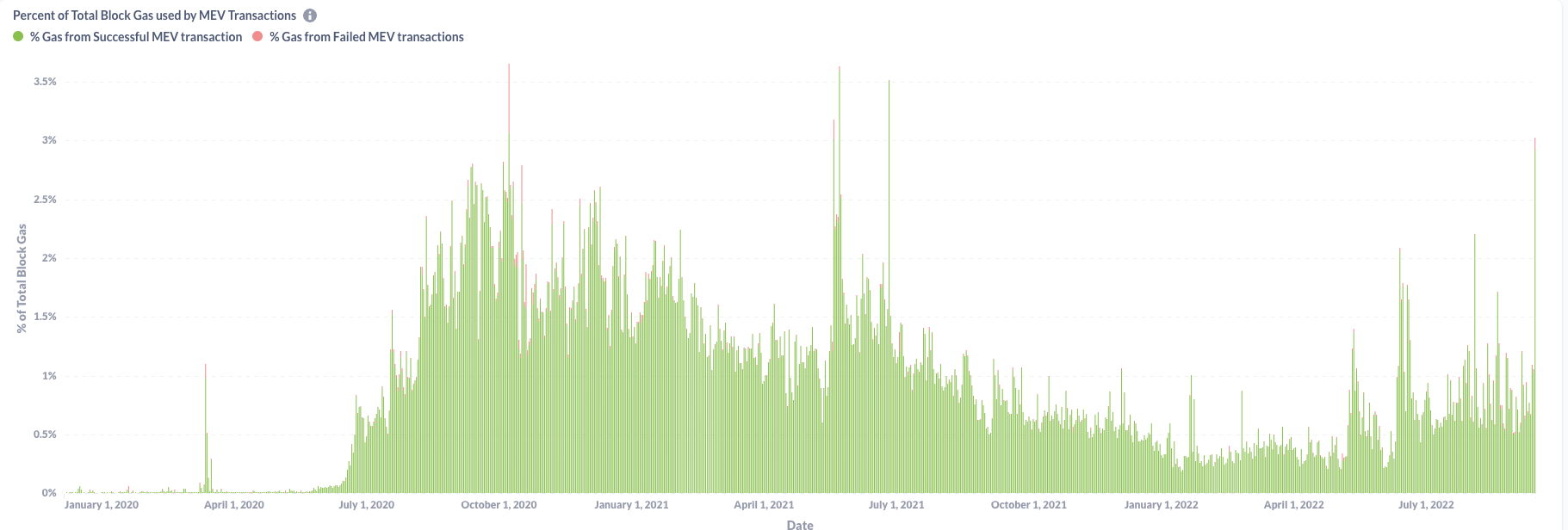
MEV extraction is a reality and almost inevitable
imposes negative externalities as e=bots bid up gas prices
"Flashbots" protocol "democratizes" exploits
protocols became better at preventing sandwich attacks with better functionality

read more at: "Battle of the Bots: Flash Loans, Miner Extractable Value and Efficient Settlement", Lehar & Parlour, 2023

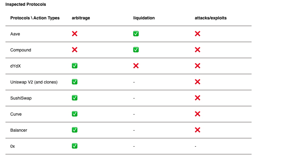
Dark side of DEx trading: Miner extractable value

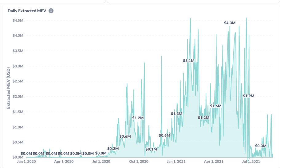
Literature

AMM Literature: a booming field

Theory
- Lehar and Parlour (2021): for many parametric configurations, investors prefer AMMs over the limit order market.
- Aoyagi and Ito (2021): co-existence of a centralized exchange and an automated market maker; informed traders react non-monotonically to changes in the risky asset’s volatility
- Capponi and Jia (2021): price volatility $\to$ welfare of AMM LPs; conditions for a breakdown of liquidity supply in the automated system; more convex pricing $\to$ lower arbitrage rents & less trading.
- Capponi, Jia, and Wang (2022): decision problems of validators, traders, and MEV bots under the Flashbots protocol.
- Park (2021): properties and conceptual challenges for AMM pricing functions
- Milionis, Moallemi, Roughgarden, and Zhang (2022): dynamic impermanent loss analysis for under constant product pricing.
- Hasbrouck, Rivera, and Saleh (2022): higher fee $\Rightarrow$ higher volume
Empirics:
- Lehar and Parlour (2021): price discovery better on AMMs
- Barbon and Ranaldo (2022): compare the liquidity CEX and DEX; argue that DEX prices are less efficient.
Math Literature: large number of papers that study AMMs in applied maths
- e.g. Cartea, Drissi, Monga (2023): closed form solution to IPL and optimizing strategy

The Bigger Picture and Last Words

Last Words

here: blockchain $\approx$ value management infrastructure
can combine asset custody, orders, trading, clearing, and settlement
allows different IO of markets and market services

AMMs are a genuinely new market institution
evolving space, new ideas come up all the time:
- UniSwap v4 is on its way
- MakerDAO's PSM is the second-most used AMM and has a completely different purpose
- may be embedded in many applications and processes
- lots to learn

bone-headed regulators and policy-makers are on route to preventing welfare-improving innovations from a variety of different angles

Decentralized Trading

Trading Infrastructure

Let's look at some stylized facts

Issues and concerns with CEX trading

Costly Arbitrage

=> arbitrage = commit capital on multiple exchanges

Volume Manipulation

Cryptocurrency Pump-and-Dump Schemes Tao Li, Donghwa Shin, and Baolian Wang, 2020

Price Manipulation: Pump & Dump

vs.

Price Manipulation: Pumping Bitcoin

Price Manipulation: Pumping Bitcoin

Security Risk

... 300 lines of code ...

Trading Infrastructure

Let's look at some stylized facts

Let's look at some stylized facts

How does it look?

automated market maker

Application: decentralized trading with automated market makers

Problem: MEMPOOL Frontrunning is intrinsically profitable

Dark side of DEx trading: Miner extractable value

Decentralized
Trading

Cryptocurrency Pump-and-Dump Schemes
Tao Li, Donghwa Shin, and Baolian Wang, 2020