Decentralized Trading 2025-26

Andreas Park

Goal of this class

ultra-brief intro to the area of market microstructure
introduction to the analysis of decentralized trading

Why care about Decentralized Trading?

Traditional Markets

What is Market Microstructure?

How do trading institutions affect market outcomes, e.g.
- trading costs
- information efficiency
- allocative efficiency
A lot of tricky issues
- no one model can do it all
- complex theoretical problems (e.g., infinite regress)
- large datasets

There are many ways to arrange trading

central limit order book

centralized auction

bilateral
negotiation

Request
for Quote

open
outcry

How hard is it to organize trading?

central limit order book

operational complexity

centralized auction

bilateral
negotiation

Request
for Quote

open
outcry

Do you know who you are trading with?

central limit order book

operational complexity

centralized auction

bilateral
negotiation

Request
for Quote

open
outcry

little

a lot

How good is the arrangement at discovering the market price?

central limit order book

operational complexity

centralized auction

bilateral
negotiation

Request
for Quote

open
outcry

bad

good

Most of the time there is no "coincidence of wants"
$\Rightarrow$ Need liquidity providers!

CoW? $\to$ Liquidity Provision

Why is there trading?
- diversification/liquidity shocks
- private information
- $\to$ Who are you providing liquidity to and what risk do you face?

For all practical purposes, modern electronic markets are organized as limit order books

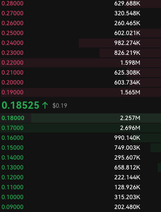
a person wants to buy $x$ shares up to price $p$

buys $x_1$ at price $p_1$
buys $x_2$ at price $p_2>p_1$
$\ldots$
buys $x_n$ at price $p_n>p_{n-1}$
pays \[\sum_{i=1}^n x_ip_i.\]

For all practical purposes, modern electronic markets are organized as limit order books

quantity

price

$Q$

$p(Q)$

$P^{\mathsf{dp}}(Q)=\int_0^Qp(q)~dq$

a person wants to buy $x$ shares up to price $p$

buys $x_1$ at price $p_1$
buys $x_2$ at price $p_2>p_1$
$\ldots$
buys $x_n$ at price $p_n>p_{n-1}$
pays \[\sum_{i=1}^n x_ip_i.\]

Some first principles insights

quantity

price

$Q$

$p(Q)$

$P^{\mathsf{dp}}(Q)=\int_0^Qp(q)~dq$

suppose someone knows that the "true value is $p(Q)$
is willing to buy for all prices $p<p(Q)$
for $Q$ the seller receives only an average price $\to$ loss

How can the liquidity provider survive?

{

the bid ask spread

Idea: earn the bid ask spread sufficiently often

every microstructure model has some form of compensation for liquidity provision

Super-quick overview over seminal papers

joint arrival at the market $\to$ no "liquidity provision"
- Grossman & Stiglitz (AER 1980)

people "buy" noisy information
demand = supply
price reveals information
marginal value of info = cost of info

competitive liquidity provider receives order flow and sets zero-profit price
noise trader order flow
monopolist informed trader cautiously trades over time to conceal info
slope of the price curve measures liquidity

risk-averse market makers require compensation for risk-taking (position risk)
liquidity-motivated traders submits order
what determines the price slope?

informed and uninformed arrive in random sequence at the market
market maker posts bid and ask prices that account for info-driven loss
what determines the spread?

submit market vs limit order?
post limit order = trading option for others
fundamental may change and may not be able to adjust limit order
gives rise to price slope and spread

trader's order $\to$ liquidity provision
- Kyle (ECTA 1985)
- Grossman & Miller (JF 1988)

liquidity provision $\to$ trader's orders
- Copeland and Galai (JF 1983)
  Glosten & Milgrom (JFE 1986)
  Glosten (JF 1994)
- Foucault (JFM 1999)

TradFi vs Crypto Trading

What makes DeFi different from TradFi?

Self-custody of assets
Access to financial infrastructure
Conceptually non-custodial, auto-executing services
Value management layer = common resource
Platform approach to commerce

{

features

consequences

Could this give us Fisher Black's vision of a fully automated stock exchange?

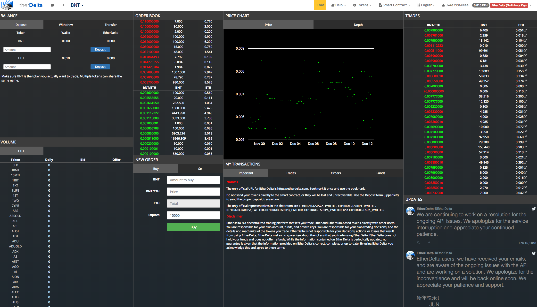
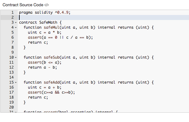
... 300 lines of code ...

Could you not just run a limit order book on a blockchain?

Actually ...

bad idea
Why?
Data-intensive, computation intensive, costly, inefficient

limit order involve many choices
isn't really "automated"

What would a minimalist automated market look like?

Two assets:
- cash and an asset
- liquidity deposits of $c$ cash and $a$ asset
self-contained market: pricing rule based on
- deposits $a,c$ and
- liquidity demanded $q$
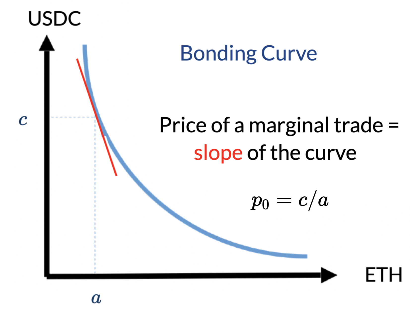
implied value of the asset at deposit: \[p=\frac{c}{a}.\]

Changes to liquidity

trades create linear changes:
- a trade of $q\in(-\infty,a),$ will cost $\Delta c(q)$
- liquidity changes
  - $a$ $\to$ $a-q$
  - $c$ $\to$ $c+\Delta c(q)$

Requirements on the marginal price

an infinitesimal unit should cost \[p^m=p\]
marginal price after trade of $q$ is \[p^m(0)=\frac{c}{a}~~\to~~p^m(q)=\frac{c+\Delta c(q)}{a-q}.\]
Marginal traded unit costs the marginal price \[\Delta c'(q)=p^m(q).\]

These minimal requirements define a pricing rule

Proposition: Consider an automated market with liquidity deposits in cash $c>0$, asset $a>0.$ Costs for a trade of $q<a$ is defined by a function $C(q):=\Delta c(q)$ that satisfies a boundary and monotonicity conditions $C(0)=0,\;C(q)>0,\;C'(q)>0$ as well as spot–marginal consistency $ C'(q)=\frac{c+C(q)}{a-q}\qquad(0\le q<a).$ Then the trading costs in this automated market is uniquely defined by
\[\Delta c(q)=q\cdot\frac{c}{a-q}~~\text{ so that }~~\Delta c'(q)=\frac{ac}{(a-s)^2}.\]

This pricing rule has a limit order book interpretation:

\[\Delta c(q)=\int_0^q \Delta c'(s)ds=\int_0^q \rho(s) ds=\int_0^q \frac{ac}{(a-s)^2} ds=q\cdot\frac{c}{a-q}.\]

A few observations

with minimal requirements we can get a pricing rule
the pricing rule looks like a limit order book
specific limit order book rule as nice properties
- it doesn't pay to split an order
- you buy $q$ and sell $q$ right after
  - same cash and assets in system
  - but cannot earn spread even though trades have price impact

Decentralized Trading

Broker

Exchange

Internalizer

Wholeseller

Darkpool

Venue

Settlement

The Basic Organization of the Market

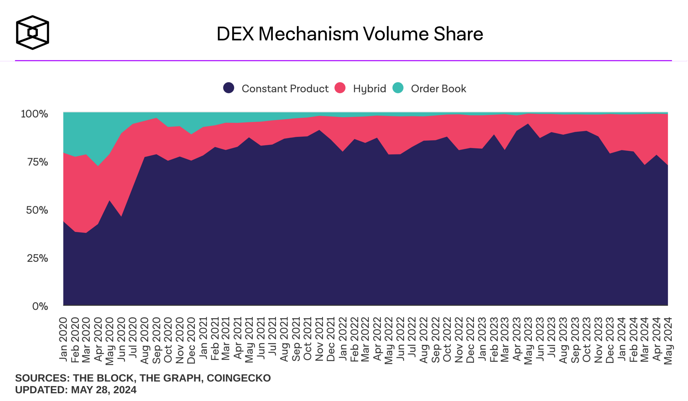
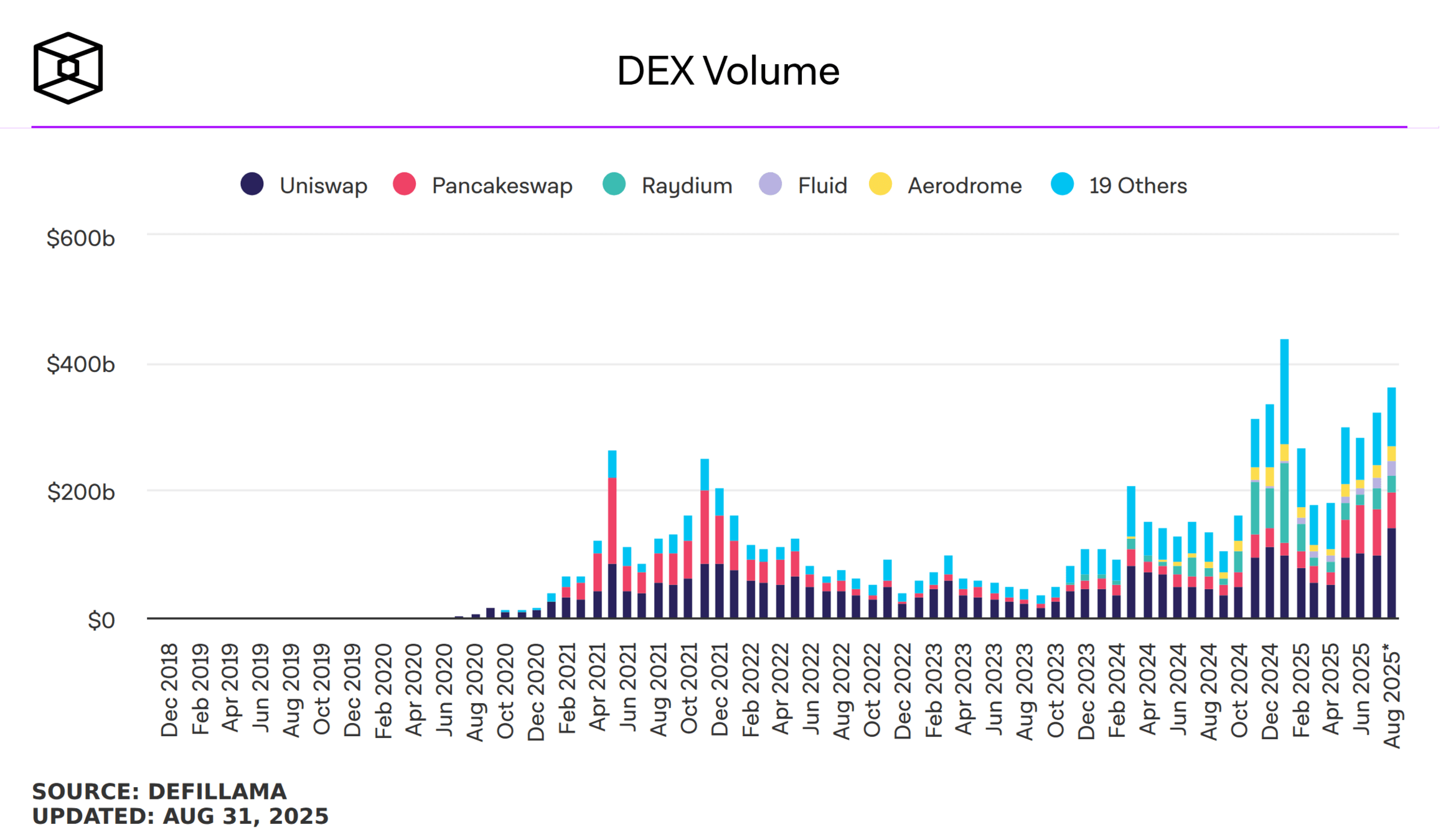
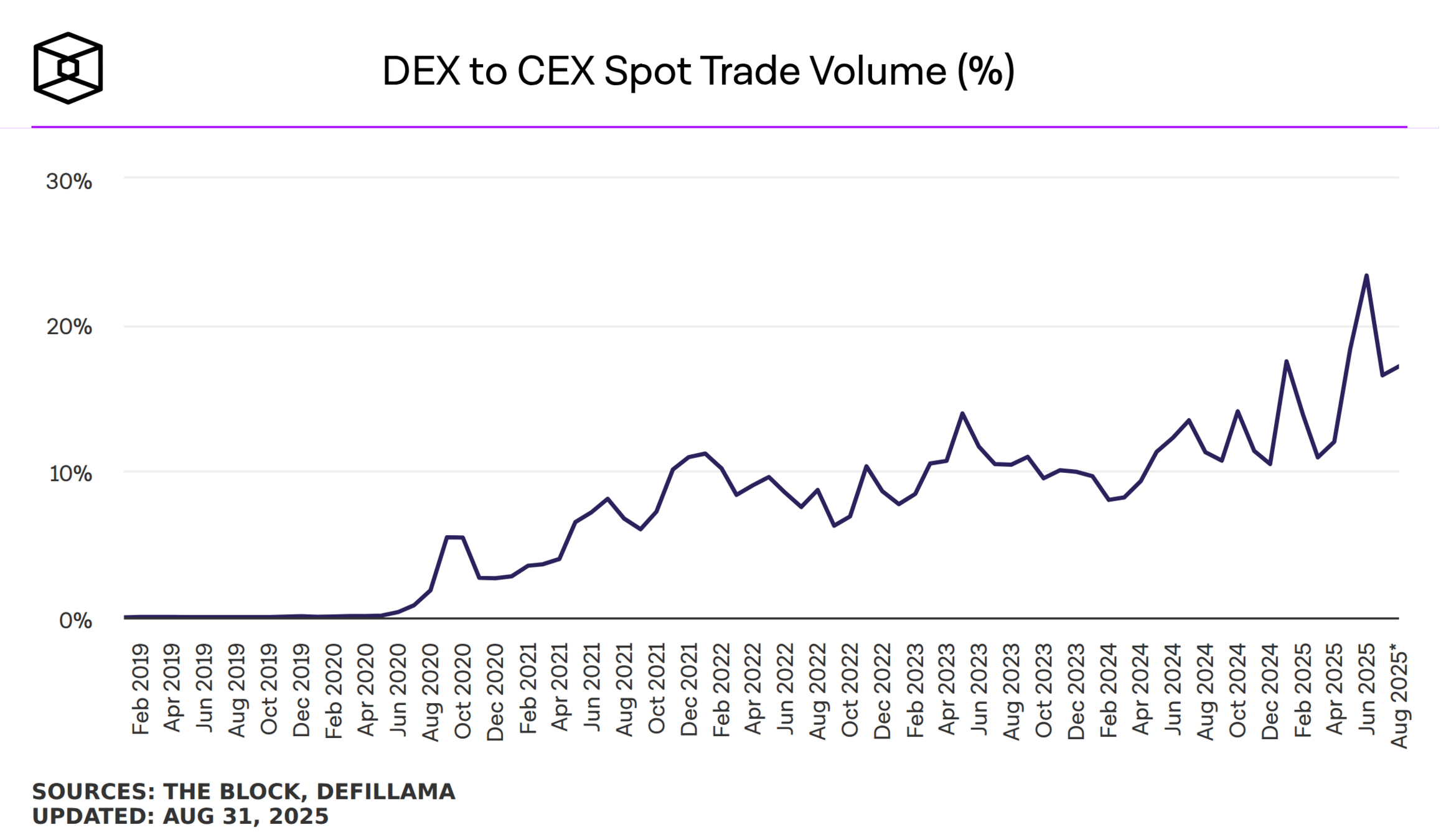
Let's look at some stylized facts

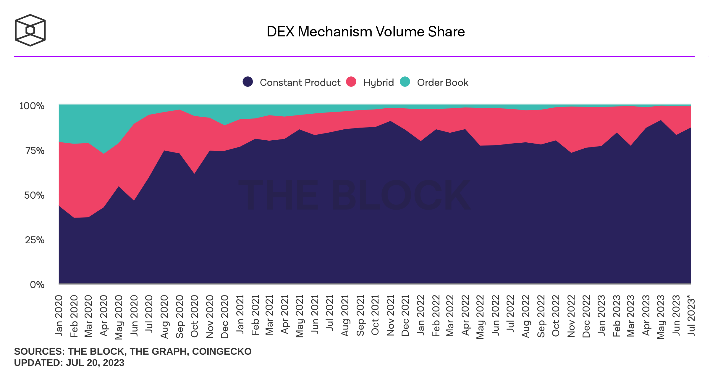
Decentralized trading using automated market makers (AMM)

Liquidity providers

Liquidity demander

Liquidity Pool

AMM pricing is mechanical:

determined by the amounts of deposits
most common:
- constant product
- #USDC $\times$ #ETH = const

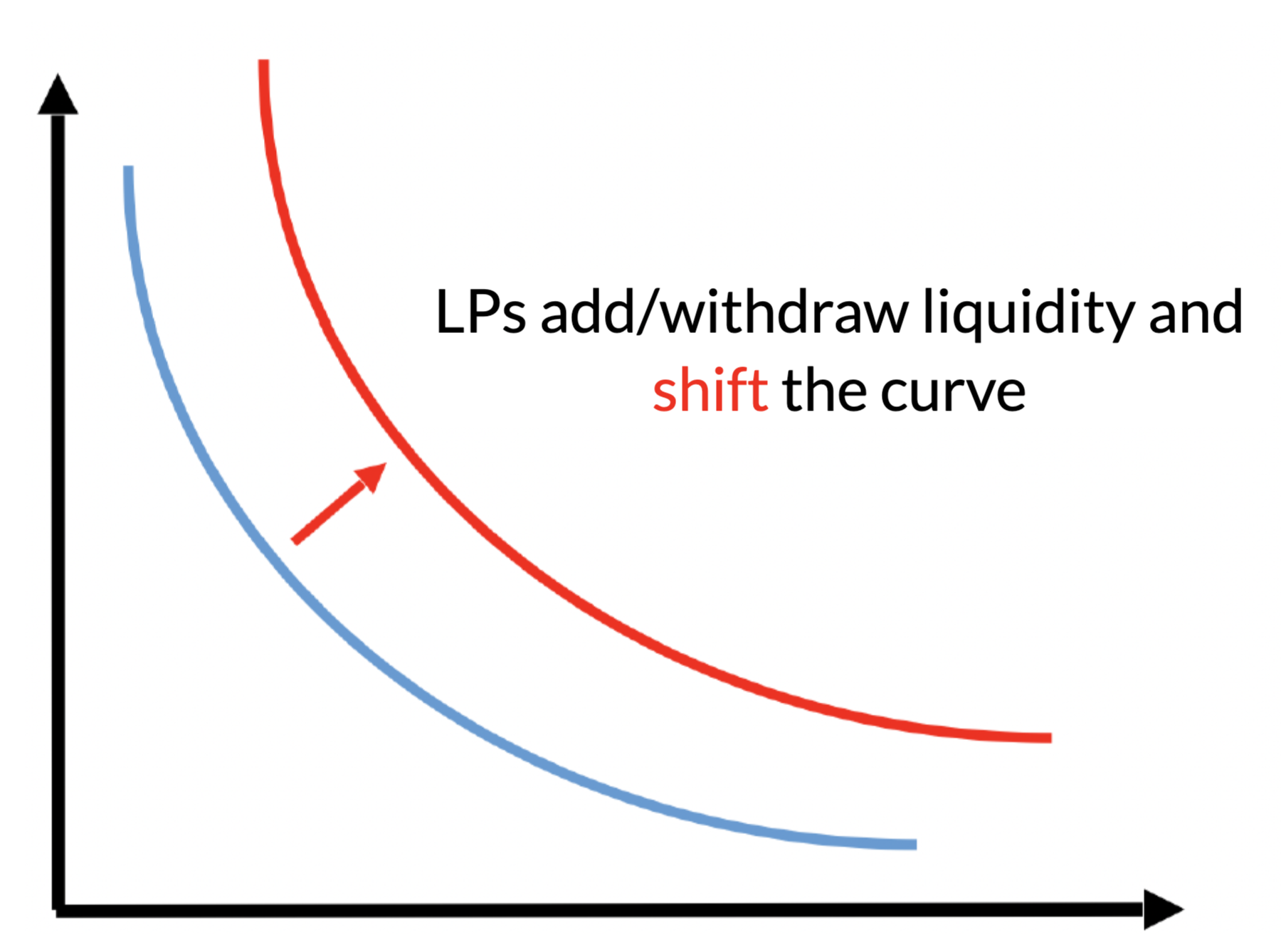
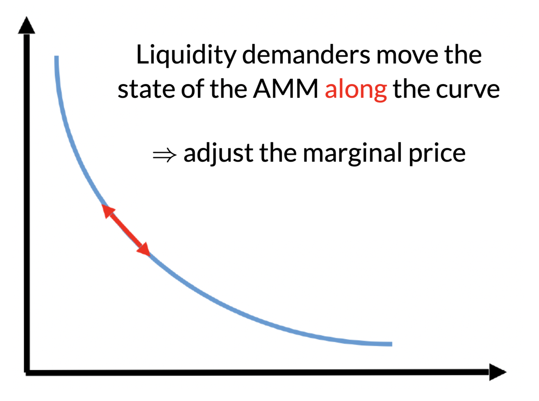
No effect on the marginal price

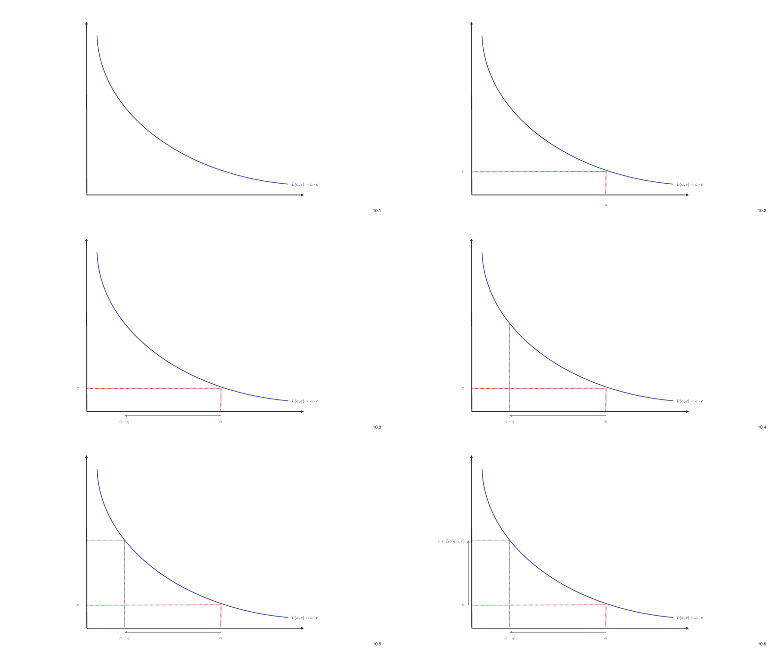
Idea of pricing: liquidity before trade $=$ after trade
\[L(a,c)=L(a-q,c+\Delta c)\]

Most Common Pricing Rule in DeFi: Constant Product

With \[a\cdot c= (a-q) (c+\Delta c(q))\]
we compute cost \[\Delta c(q)=q\cdot \frac{c}{a-q},\]
and marginal price \[p^m(q)=\frac{c+\frac{cq}{a-q}}{a-q}=\frac{ac}{(a-q)^2}.\]

Insight: AMM pricing function is the same as a limit order book when we require

that prices are continuous and
that prices are determined by liquidity deposits only

limit order book: \[p(q)=\frac{c}{a-q}.\]
constant product: \[p(q)=\frac{c}{a-q}.\]

The Pricing Function

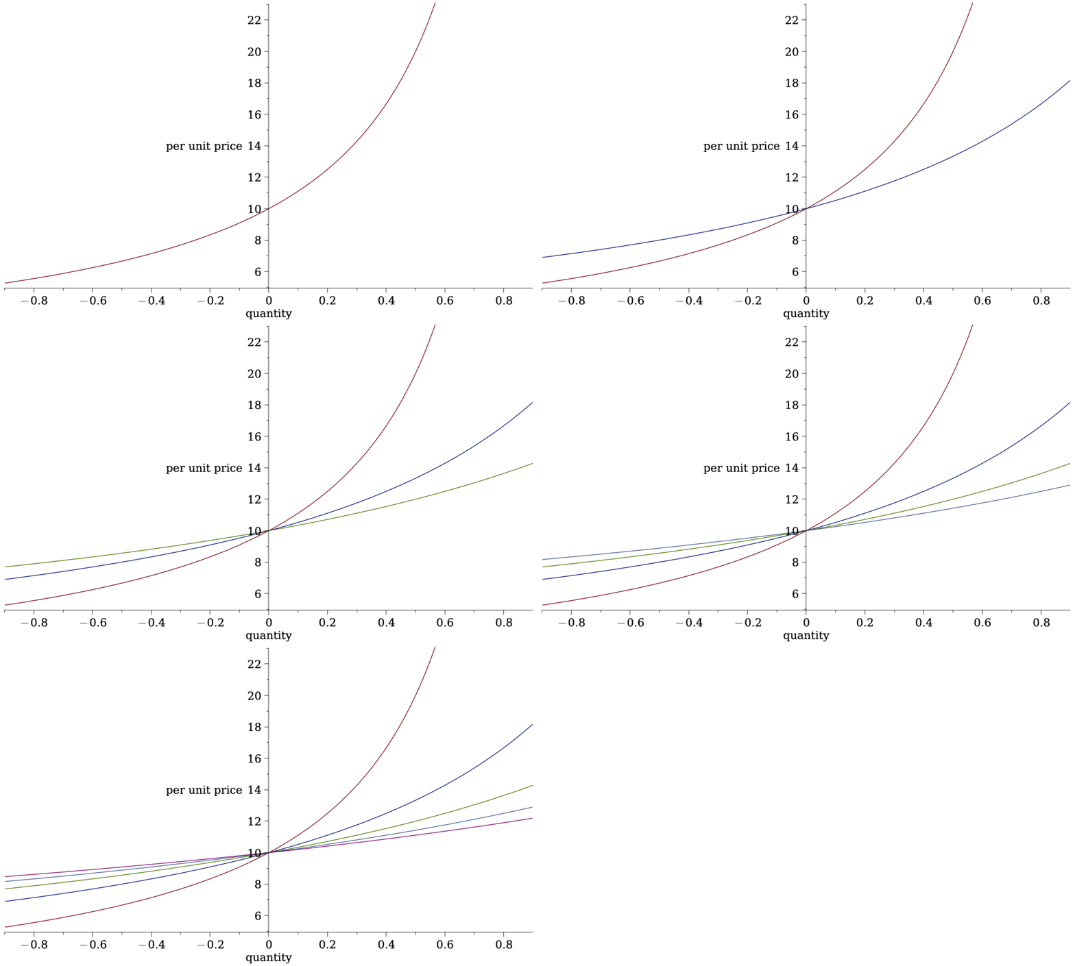
An Alternative Pricing Function

Some Pricing Rules from Traditional Markets: Uniform Price

assume cost is price $\times$ quantity: \[\Delta c(q)=q\cdot p^m(q)\]
plus assume average price $=$ marginal price after trade

\[p^m(q)=\frac{c+q\cdot p^m(q)}{a-q}~~\Leftrightarrow~~p^m(q)=\frac{c}{a-2q}.\]
(This is essentially how opening auctions, open outcry etc work and how models like Kyle (1985) and Grossman-Miller (1980) work)
formalized and analyzed by Canidio and Fritsch (2023) and implemented in COW-Swap

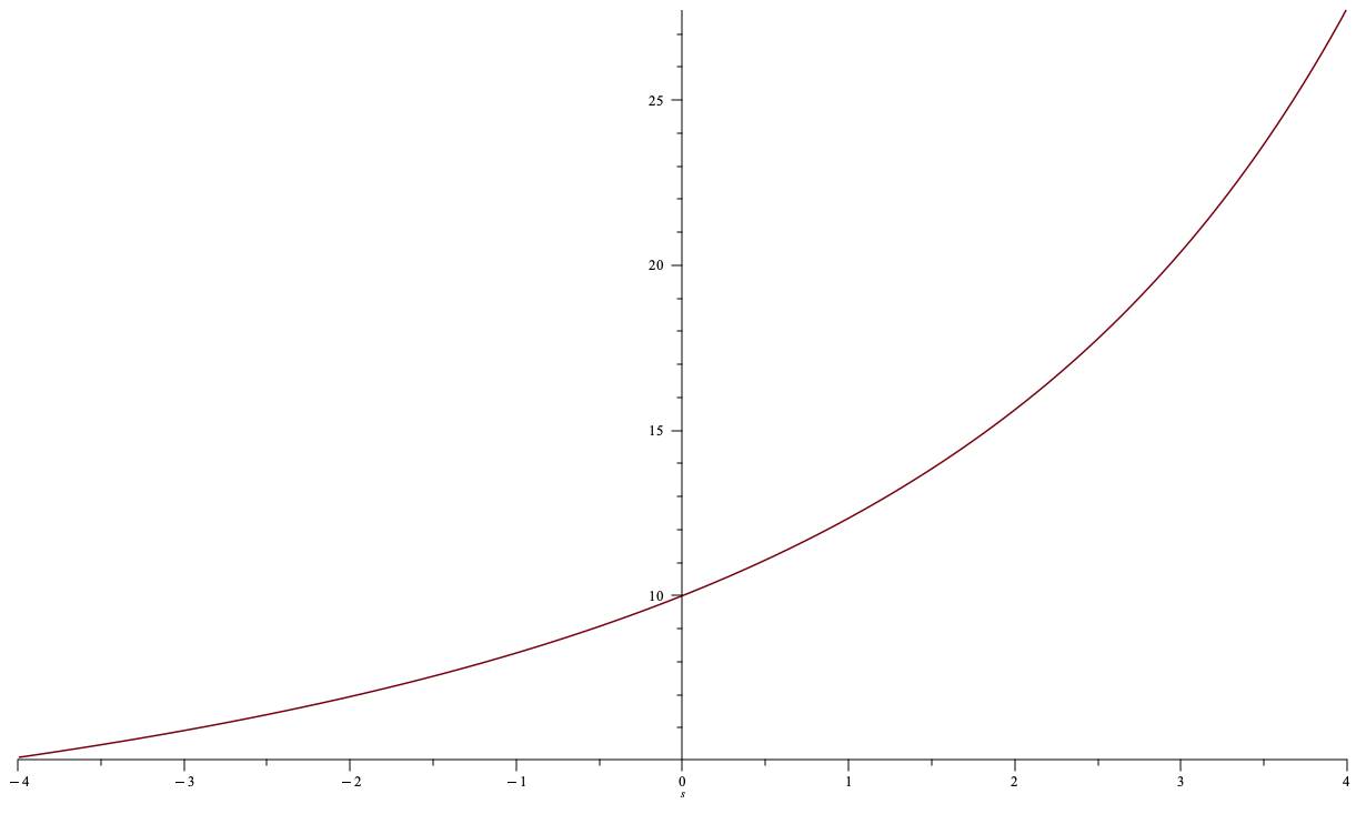
$q=2$

$\Delta c(q)= q\times p^m(q)=2\times 15.5$

Some insights on pricing functions

Price $\times$ quantity
- nice feature:
  - regret-free price: if price move is due to information, you have no positional loss
- poor feature:
  - you can always save by order-splitting (formally shown by Canidio and Fritsch (2023))
  - limit if slice $\to$ 0 = limit order book price

Constant Product
- nice feature:
  - order splitting doesn't pay
  - has a limit order book interpretation
  - canonic implementation of automated trading
- poor feature:
  - prices not regret-free: if price move is due to information, you always lose

UniSwap v3

UniSwap v3 has "concentrated liquidity provision"

liquidity provision choice in v2:
- submit $a,c$ at the marginal $p_0=\frac{c}{a}$
- $\to$ for given $p_0$, there is ONE degree of freedom
- provide liquidity
  - for all prices $p\in(0,\infty)$
  - all asset amounts $q\in(0,a)$
  - all cash amounts $\Delta c\in (0,c)$

liquidity provision choice in v3:
- submit $u,\Delta c (d)$
- choose price range $[p_d,p_u]$
- provide liquidity
  - for all prices $p\in[p_d,p_u]$
  - all asset amounts $q\in(0,u)$
  - all cash amounts $\Delta c\in (0,\Delta c(d))$

Just a little more institutional details

users submit liquidity positions $(u,d,p_u,p_d)$ and receive an ERC-721 (=NFT) token as a receipt
the code segments liquidity into discrete exponential intervals $[p_k,p_{k+1}]$ with \[p_k=(1+\delta)^k. ~~~(\text{numerically: }p(k)=1.0001^k)\]
it aggregates liquidity over these intervals
the pricing curve for each interval is determined by the constant product rule
intervals may be "empty"

How the price is determined

if the marginal price reaches the upper bound $p_u$, you will sell $u$ units of the asset
if the marginal price reaches the lower bound $p_d$, you will sell $d$ units of the cash

the price is still using constant product
virtual liquidity = v2 liquidity that would pertain if you'd supply liquidity on the entire interval of prices
constant product $\Rightarrow$ marginal price curve has functional form \[p^m(q)=\frac{\tilde{a}c}{(\tilde{a}-c)^2}\]

where $\tilde{a}$ is the virtual liquidity

quick disclaimer: what follows is not how UniSwap is explained on its website etc. But the resulting maths are the same

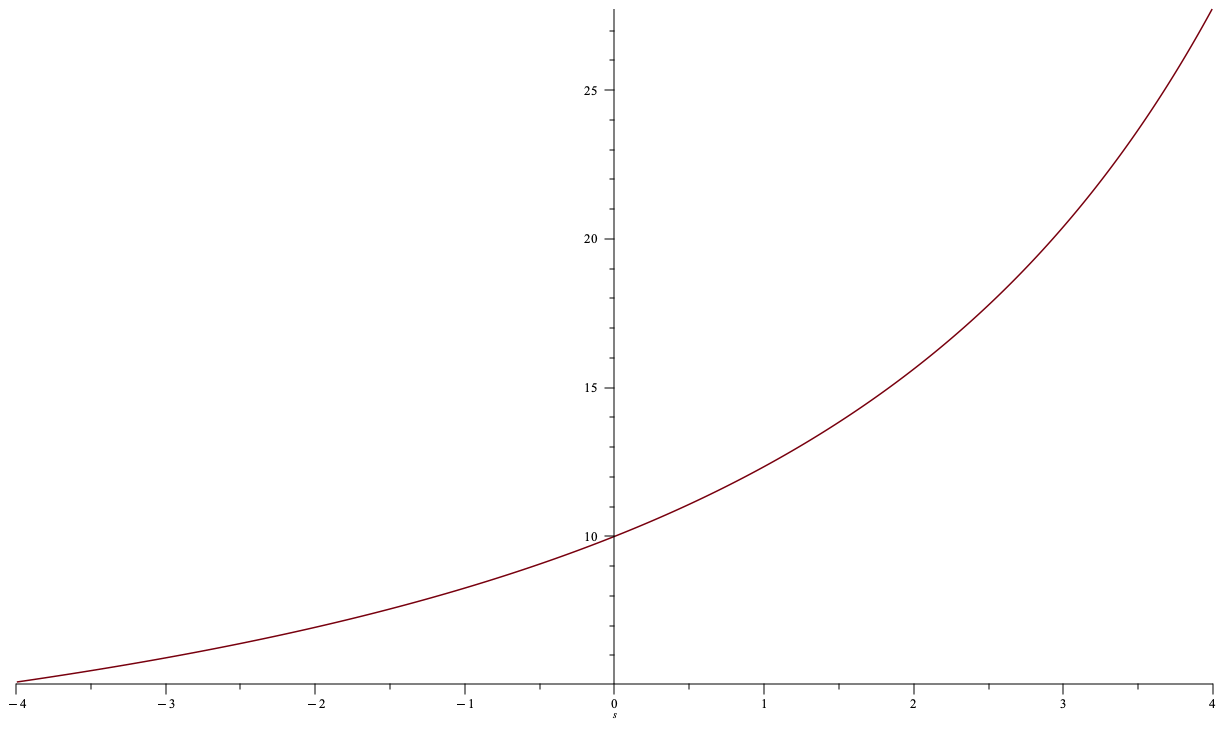
$p_d$

$p_u$

$p_0$

UniSwap v3: An Example

$p_u=15$

$p_d=7$

$u=2$

$p_0=10$ (that's exogenous, not a choice)

marginal price

\[\gamma(s)=\frac{\tilde{a}c}{(\tilde{a}-s)^2}.\]

Finding virtual liquidity factor $\tilde{a}$

marginal price

\[\gamma(s)=\frac{\tilde{a}c}{(\tilde{a}-s)^2}.\]

$p_u=15$

$p_d=7$

$u=2$

$p_0=10$ (that's exogenous, not a choice)

= find the right curve

= find the right "$\tilde{a}$"

= find $\tilde{a}$ such that \[\gamma(u)=p_u\]

Finding the fourth parameter $\Delta c(d)$

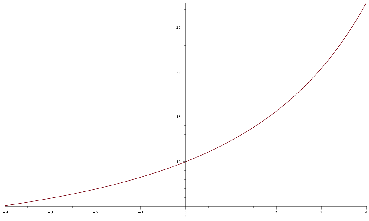
$p_u=15$

$p_d=7$

$u=2$

$d=?$

required cash deposit $\Delta c(d)=$ the amount that I pay for $d$

marginal price

\[\gamma(s)=\frac{\tilde{a}c}{(\tilde{a}-s)^2}.\]

Given $\tilde{a}$ solves $\gamma(u)=p_u$, we

solve $\gamma(d|\tilde{a})=p_d$ for $d$
determine $\Delta c(d|\tilde{a})=$ the required cash

Solutions

virtual liquidity factor: \[\tilde{a}=\frac{u}{1-\sqrt{p_0/p_u}}=u\cdot \frac{\sqrt{p_u}}{\sqrt{p_u}-\sqrt{p_0}}.\]

required quantity to reach $p_d$ \[\rho(-\tilde{d})=\frac{\tilde{a}\tilde{c}}{(\tilde{a}+\tilde{d})^2}=p_d.~~\Leftrightarrow~~d^*=-\tilde{a}(1-\sqrt{p_0/p_d})\]

required cash deposit \[\Delta c(\tilde{d})=-\tilde{a}(1 - \sqrt{p_0/p_d})\sqrt{p_0p_d}=-u\sqrt{p_0p_d}\frac{1 - \sqrt{p_0/p_d}}{1 - \sqrt{p_0/p_u}}\]

marginal pricing function \[\tilde{\gamma}(q)=\frac{\tilde{a}^2p_0}{(\tilde{a}-q)^2}=\frac{u^2p_0p_u}{((u-q)\sqrt{p_u}+q\sqrt{p_0})^2}.\]

For those in the know: These formulae/solutions are exactly the same as those in the UniSwap v3 whitepaper

Numerical example

Suppose $p_0=\$10$.
LP is willing to sell up to $u=100$
v2 liquidity:
- Required cash deposit: $c=100\times 10=1000$
- liquidity $c\cdot a=100\times 1,000$

For v3: suppose willing to supply liquidity in $[\$9,\$11]$
v3 liquidity:
- virtual liquidity factor: $\tilde{a}\approx 2,150$
- required cash $c^*=\$1,100$

consider a buy order of $q=10$
cost per unit
- v2: $\frac{1000}{100-10}=11.11$
- v3: $\frac{21,500}{2,150-10}=10.05$

Want to read more?

A Primer on UniSwap v3 Math: As Easy as 1,2, v3 https://blog.uniswap.org/uniswap-v3-math-primer
Elts 2012: Liquidity Math in UniSwap v3

Liquidity Supply and Demand in an Automated Market Maker

Facts about modelling liquidity provision

You provide liquidity when the marginal price at the AMM and elsewhere is $p(t_0)=p.$
You make a decision what to do next at $t_1>t_0$
Many things can happen, for instance:
- There was no trade on the AMM but the price on another market has moved.
- There have been trades on the AMM but the AMM price is different from prices elsewhere.
- There have been trades on the AMM and the AMM price is that same as prices elsewhere.

Each case has a different interpretation and each has been used in some form in the literature.

Key questions:

Is there arbitrage?
Is one of the prices "correct"?
What has happened between $t_0$ and $t_1$?

Some first principles insights

quantity

price

$Q$

suppose $p(Q)$

= true value

$P^{\mathsf{dp}}(Q)=\int_0^Qp(q)~dq$

market maker gets this triangle

but its worth $Q\times p(Q)$

Provide-and-Forget Liquidity Provision

Basic idea of liquidity provision: earn more on balanced flow than what you lose on price movement

\[\frac{\text{income}}{\text{capital committed}}\ge -\frac{\text{positional loss}}{\text{capital committed}} + \text{cost of capital} \]

in AMMs:
protocol fee

in tradFi: bid-ask spread

Provide-and-Forget Liquidity Provision

for given return $R$ this is a function: $\sqrt{R}-\frac{1}{2}(R+1)$

this is the choice parameter: more liquidity, smaller left hand side of the equation

\[\text{fee}\times\left(\frac{\text{expected noise volume}}{\text{liquidity deposit}}+\frac{\text{expected volume from arbitrageurs}}{\text{liquidity deposit}}\right)\ge \frac{\text{expected positional loss}}{\text{liquidity deposit}}\]

for given return $R$ this is a function: $|\sqrt{R}-1|/2$

Sidebar: we can quantify how much a PASSIVE LP loses when the price moves by $R$

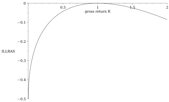
for orientation:

If the stock price drops by 10% the incremental loss for liquidity providers is 13 basis points on their deposit
- $\to$ total loss=-10.13%
If the stock price rises by 10%, the liquidity provider gains 12 basis points less on the deposit
- $\to$ total gain =9.88%

\[\frac{\text{adverse selection loss when the return is $R$}}{\text{initial deposit}}=\sqrt{R}-\frac{1}{2}(R+1)\]

see Barbon & Ranaldo (2022)

adverse selection loss
(or: impermanent loss)

Liquidity Demander's Decision & (optimal) AMM Fees

Two opposing forces in equilibrium for fee $F\nearrow$
1. more liquidity provision
  $\to$ lower price impact
2. more fees to pay

Result:

competitive liq provision$\to$ there exists an optimal (min trading costs) fee $>0$

$\to$ derive closed form solution for competitive liquidity provision
depends on return distribution, balanced volume, quantity demanded

Similar to Lehar&Parlour (2023) and Hasbrouck, Riviera, Saleh (2023)

For trading of a fixed quantity:

\[\text{LD cost}=\text{AMM price impact} +\text{AMM fee} .\]

\[F^\pi=\frac{1}{E[|\sqrt{R}-1|]+V}\left(-2q\ E[\text{position loss}]+ \sqrt{-2qV\ E[\text{position loss}]}\right).\]

assume: liquidity providers add liquidity until they break even in expectation

Fee = Liquidity Measure ... with approximations

\[F^\pi=\frac{1}{E[|\sqrt{R}-1|]+V}\left(-2q\ E[\text{position loss}]+ \sqrt{-2qV\ E[\text{position loss}]}\right).\]

\[F^\pi\approx\frac{|r|}{2\sqrt{N}}.\]

for volume $V$ large
quantity $q=V/N$ with $N$ number of transactions

for lognormal $R$ with mean 1 and variance $\sigma^2$

\[F^\pi\approx\frac{\sigma}{2\sqrt{N}}.\]

price impact $\approx F^\pi$

also for large $V$

recall the Amihud measure of illiquidity \[\ell=\frac{|r|}{DV}\]
but ... Amihud is purely an empirical heuristic
this here is microfounded

Liquidity Provision as Options

Liquidity = give others the option to trade
Limit order book: (Copeland & Galai JF 1983) liquidity provision $=$ is a short strangle: call at the ask, put at the bid
Hasbrouck, Riviera, Saleh (MS 2025): AMM v3 Liquidity Provision is a covered call
- long in the underlying (when price drops, they hold the asset)
- sell a call (when the price rises, their payoff is as if writng a call)
- earn fees (premium) when the price is below the strike
Milionis, Moallemi, Roughgarden, and Zhang (2022): A LVR strategy has several analogies in options pricing
- it's a bit like a protective put: rebalancing protects against losses
- it's a bit like Delta-Hedging to stay neutral to price movements

Ciamac Moallemi will explain details later!

Empirical Work

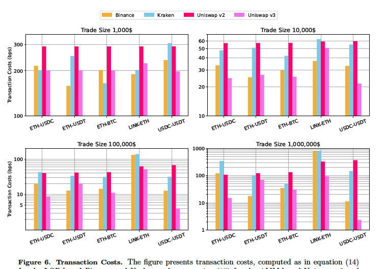
Lehar and Parlour (2021)

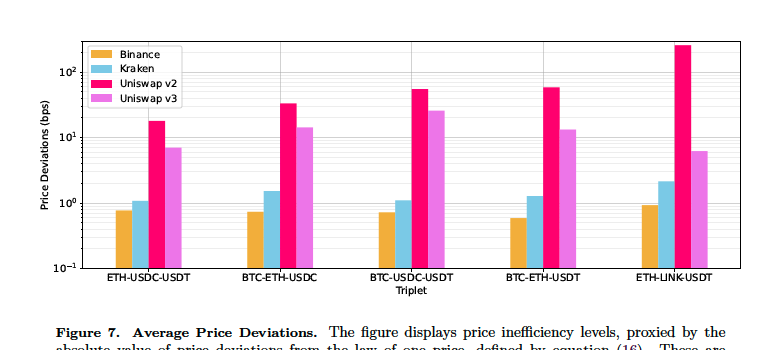
Barbon & Ranaldo (2023)

Other notables:

Lehar, Parlour, Zoican (2022):
- study and document fragmentation of liquidity across different fee levels
- most intense provision-withdrawal activity for low fees $\to$ UniSwap v3 starts mimicking tradfi
Capponi & Jia (2022) study impact of curvature of pricing function
- Theory: curvature of optimal pricing curve $\nearrow$ volatility
- Empirics: cost volatility is 60% lower for stable-coin pairs
- corr(deposit inflows ,volatility)<0
  corr(deposit inflows ,volume)>0

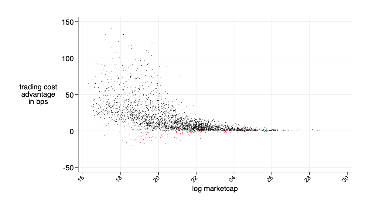
Malinova & Park (2023): AMM applied to equities would reduce trading costs by 30%

Concerns around Automated Market Makers

a

b

c

d

e

f

g

Problem 1: Sandwich (MEV) attacks

related paper: “Maximal Extractable Value and Allocative Inefficiencies in Public Blockchains”. A. Capponi, R. Jia, and Y. Wang (2023)

With v2 AMM pricing, losses are arbitrarily large (Park 2023)
Slippage protection can mitigate losses but comes with execution risk

NB: PBS does not solve the problem

a

b

c

d

e

f

g

Problem 2: Arbitrage Trades that Reduce LVR

Key LVR Idea:
- rebalancing benefits liquidity providers
- allows lower equilibrium fees

PBS creates the problem

builder/searcher

Arbitrage
- reduces rebalancing benefits
- $\to$ eliminates the fee advantage
- $\to$ increases equilibrium fees

Problem 3a: Just-In-Time Liquidity (single trade cream skimming)

X-Router

Liquidity pool

OTC

Problem 3b: Just-In-Time Liquidity (at the builder/MEV level)

X-Router

Liquidity pool

searcher/builder

balanced orders

add as much liquidity as possible

withdraw liquidity

unbalanced orders

the issue:
- order flow segmentation increases adverse selection
- JIT: not enough fees from balanced order flow

related paper: Capponi, Jia, and Zhu (2024) "The Paradox of Just-in-Time Liquidity in Decentralized Exchanges: More Providers Can Lead to Less Liquidity"

Other things

v2 is simple, v3 is complex and closer to LOB, v4 fragments liquidity
- $\to$ is the long run going to be high activity LOB?
- how (well) is liquidity aggregated across systems?
can a simple setting compete with a complex setting (is the fully-spec'ed LOB still inevitable?)
multi-coin liquidity models
AMMs as investment income add-ons and their role in capital raising

The Bigger Picture and Last Words

Last Words

AMMs are a genuinely new market institution
evolving space, new ideas come up all the time:
- UniSwap v4 is here - can it solve the problems?
- may be embedded in many applications and processes
- lots to learn
Will we re-discover and re-create many of the problems of existing markets?

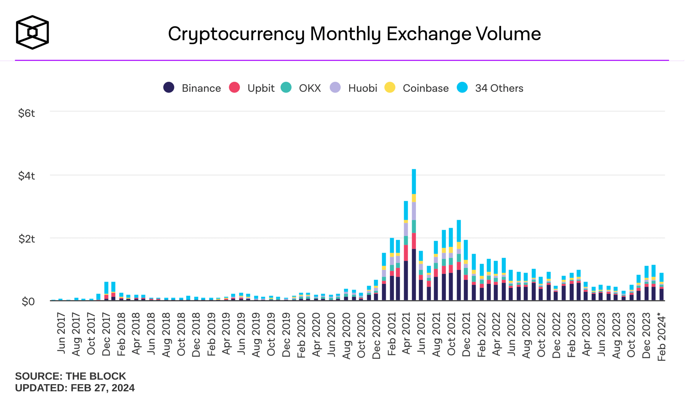
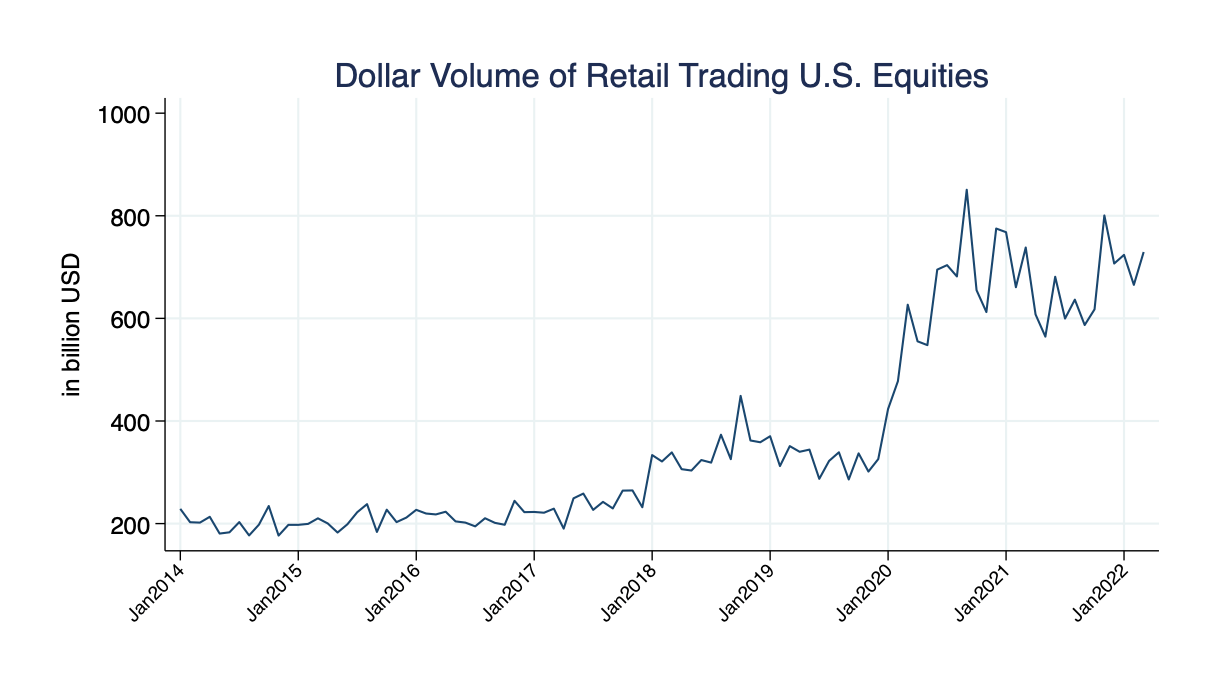
data: authors calculations from TAQ (up to March 2023)
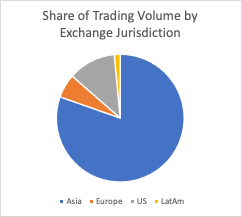
crypto volume worldwide is larger than US retail by factor >4

Decentralized Trading 2025-26

... 300 lines of code ...

Could you not just run a limit order book on a blockchain?

Let's look at some stylized facts

Decentralized trading using automated market makers (AMM)

How do people trade on-chain?