DESI 2024: Survey overview and first cosmological results
Arnaud de Mattia - CEA Saclay
Hendaye, August 23rd
- physics motivation
- the survey
- first results
- what's next?

DESI maps galaxies
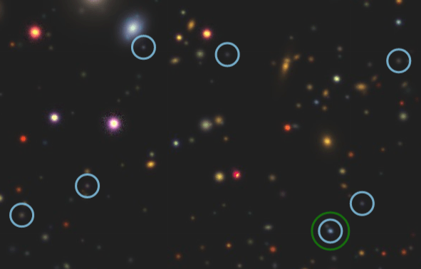
- photometric surveys provide angular positions of galaxies
R.A.
Dec.

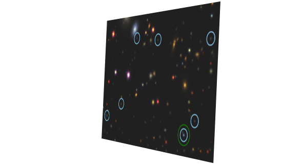
DESI maps galaxies
- photometric surveys provide angular positions of galaxies
- spectroscopic measurements for the redshift (radial) dimension

R.A.
Dec.
R.A.
Dec.
z

DESI 3D Map
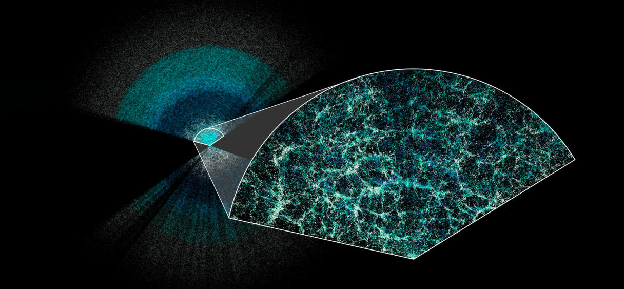
Physics program
- Galaxy and quasar clustering
- Lyman-alpha forest
- Clusters and cross-correlations
- Galaxy and quasar physics
- Milky Way Survey
- Transients and low-z

DESI 3D Map

Physics program
- Galaxy and quasar clustering
- Lyman-alpha forest
- Clusters and cross-correlations
- Galaxy and quasar physics
- Milky Way Survey
- Transients and low-z

Clustering measurements
2-pt correlation function \(\xi(s)\): excess probability of finding two galaxies seperated by a given separation \(s\)
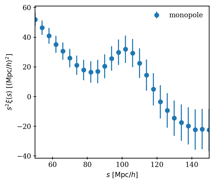

Clustering measurements
2-pt correlation function \(\xi(s)\): excess probability of finding two galaxies seperated by a given separation \(s\)
Power spectrum \(P(k) = \mathrm{FT}(\xi(s))\)

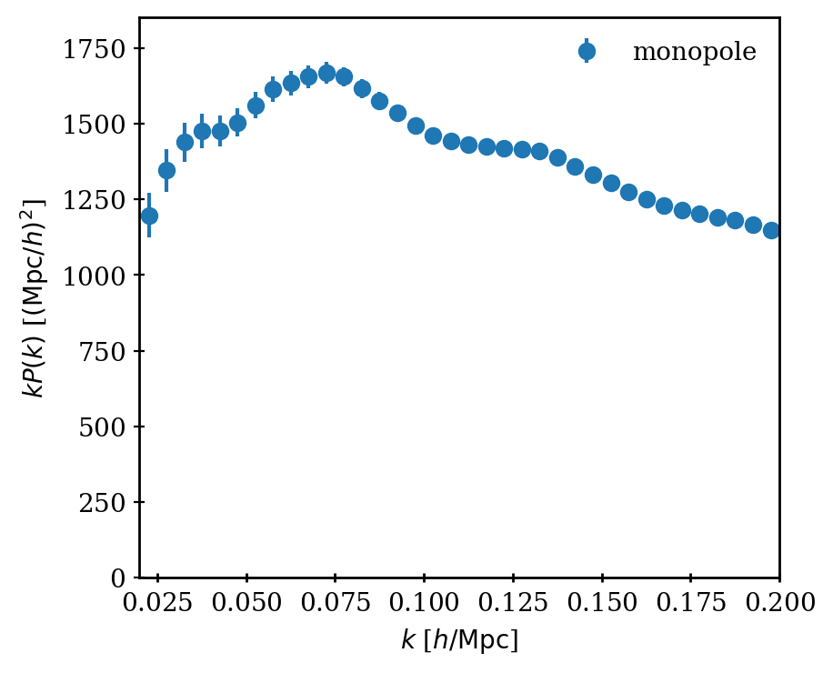

Baryon acoustic oscillations
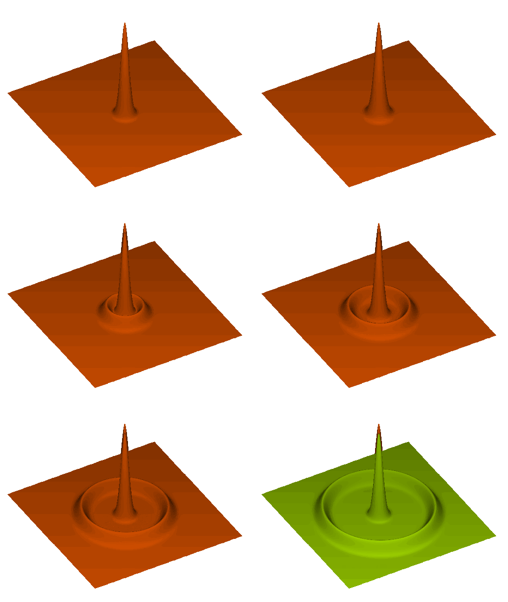
Sound waves in primordial plasma
At recombination (\(z \sim 1100\))
- plasma changes to optically thin
- baryons decouple from photons
- sound wave stalls

Baryon acoustic oscillations

Sound waves in primordial plasma
spherical shell in the distribution of galaxies, of radius the distance that sound waves travelled
= sound horizon scale at the drag epoch \( r_\mathrm{d} \sim 150 \; \mathrm{Mpc} \sim 100 \; \mathrm{Mpc}/h \)
At recombination (\(z \sim 1100\))
- plasma changes to optically thin
- baryons decouple from photons
- sound wave stalls

Baryon acoustic oscillations

Sound waves in primordial plasma
spherical shell in the distribution of galaxies, of radius the distance that sound waves travelled
= sound horizon scale at the drag epoch \( r_\mathrm{d} \sim 150 \; \mathrm{Mpc} \sim 100 \; \mathrm{Mpc}/h \)
At recombination (\(z \sim 1100\))
- plasma changes to optically thin
- baryons decouple from photons
- sound wave stalls
standard ruler

- transverse to the line-of-sight: \(D_\mathrm{M}(z) / r_\mathrm{d}\)

BAO measurements
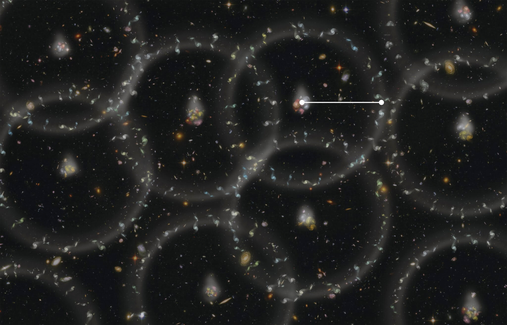
transverse comoving distance
sound horizon \(r_d\)

- transverse to the line-of-sight: \(D_\mathrm{M}(z) / r_\mathrm{d}\)
- along the line-of-sight: \(D_\mathrm{H}(z) / r_\mathrm{d} = c / (H(z) r_\mathrm{d}) \)
BAO measurements


Hubble distance
sound horizon \(r_d\)

- transverse to the line-of-sight: \(D_\mathrm{M}(z) / r_\mathrm{d}\)
- along the line-of-sight: \(D_\mathrm{H}(z) / r_\mathrm{d} = c / (H(z) r_\mathrm{d}) \)
At multiple redshifts \(z\)
BAO measurements


Probes the expansion history, hence the energy content (DE)
Absolute size at \(z = 0\): \(H_0 r_d\)
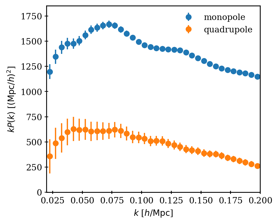
Full shape analysis

observed redshift = Hubble flow

Full shape analysis

observed redshift = Hubble flow and peculiar velocities (RSD = "redshift space distortions")

Full shape also driven by primordial physics (\(\omega_m, \omega_b, n_s, f_{\mathrm{NL}}, ...\))
RSD probes growth of structure \(f\sigma_8\), sensitive to gravity, DE, \(\nu\)


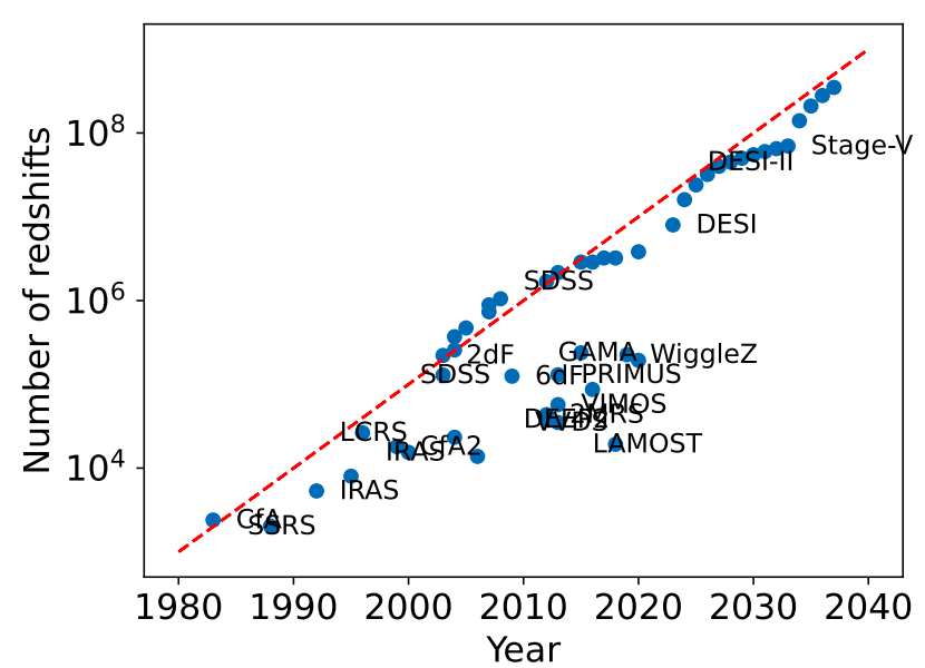
DESI: a stage IV survey
DESI vs SDSS

| Mirror diameter | 2.5 m | 4 m |
| Number of fibers | 1000 | 5000 |
| Troughput | ~20% | 20%-50% |
| Spectro resolution | 1560 - 2650 | 2000 - 5000 |


x20 survey speed and x2 resolution!

DESI Y5 galaxy samples
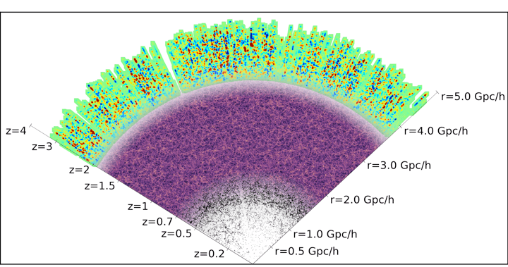
Bright Galaxies: 14M (SDSS: 600k)
0 < z < 0.4
LRG: 8M (SDSS: 1M)
0.4 < z < 0.8
ELG: 16M (SDSS: 200k)
0.6 < z < 1.6
QSO: 3M (SDSS: 500k)
Lya \(1.8 < z\)
Tracers \(0.8 < z < 2.1\)
Y5 \(\sim 40\)M galaxy redshifts!
\(z = 0.4\)
\(z = 0.8\)
\(z = 0\)
\(z = 1.6\)
\(z = 2.0\)
\(z = 3.0\)

DESI Y5 forecasts

Survey Validation (DESI Collaboration, arXiv:2306.06307)
BAO and RSD constraints at the end of the survey (\( \Delta z = 0.1 \))
Ly\(\alpha\)

DESI Y5 forecasts

Survey Validation (DESI Collaboration, arXiv:2306.06307)
BAO and RSD constraints at the end of the survey (\( \Delta z = 0.1 \))
Ly\(\alpha\)

(w/ Planck)
Thanks to our sponsors and
72 Participating Institutions!


Thanks to our sponsors and
72 Participating Institutions!

900 researchers


DOE funds the DESI project:
- operations ($12M/year)
- construction ($56M)


DOE funds the DESI project:
- operations ($12M/year)
- construction ($56M)
+ other sources ($19M, inc. in kind)
= $75M


Lawrence Berkeley National Lab (LBNL) is the managing laboratory
LBNL hosts NERSC, the computing facility for data processing


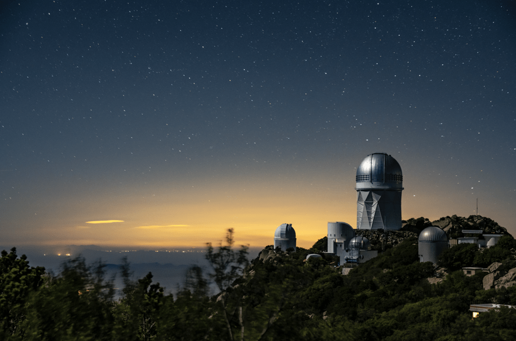
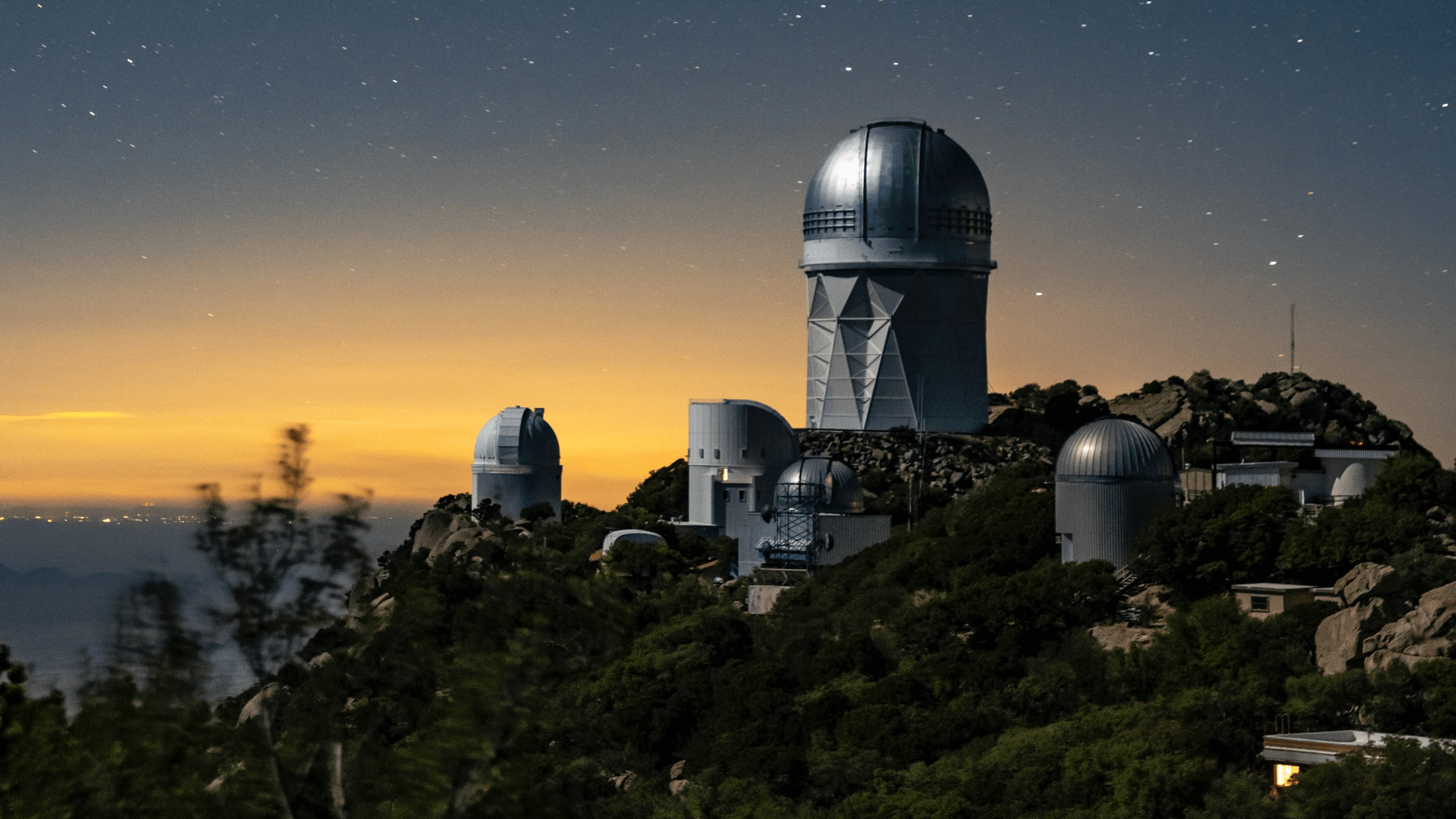
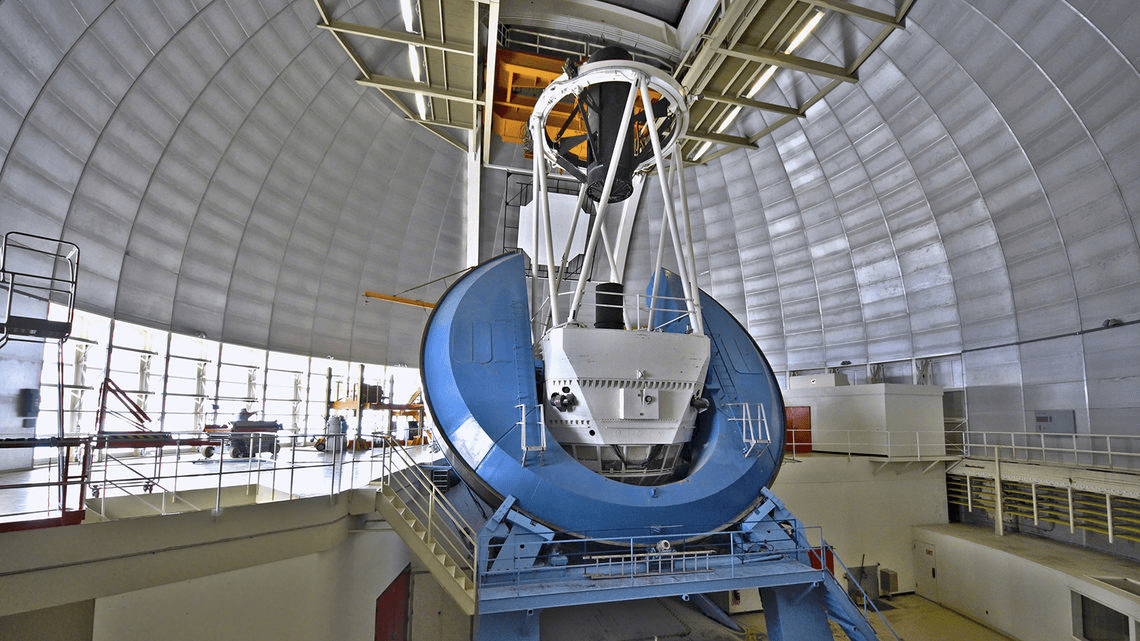
Mayall telescope at Kitt Peak National Observatory near Tucson, Arizona
Part of the NSF’s National Optical-Infrared Astronomy Research Laboratory (NSF’s OIR Lab)
The DESI collaboration is honored to be permitted to conduct scientific research on oligam Du’ag, a mountain with particular significance to the Tohono O’odham Nation.
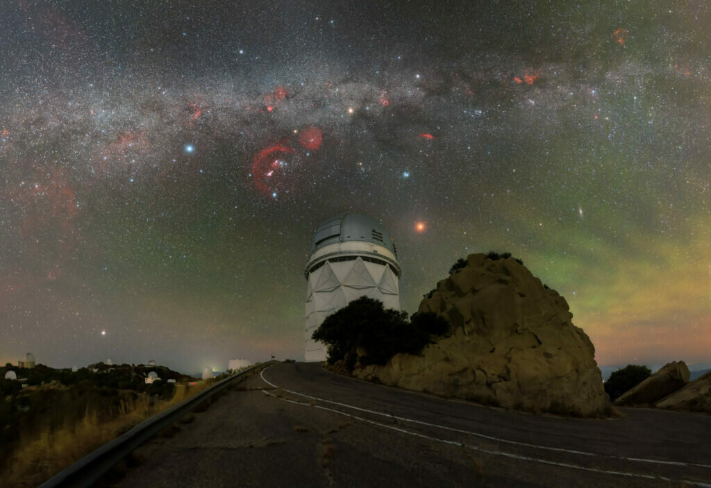
Credit: KPNO/NOIRLab/NSF/AURA/P. Horálek (Institute of Physics in Opava)

The DESI collaboration is honored to be permitted to conduct scientific research on oligam Du’ag, a mountain with particular significance to the Tohono O’odham Nation.

Credit: KPNO/NOIRLab/NSF/AURA/P. Horálek (Institute of Physics in Opava)
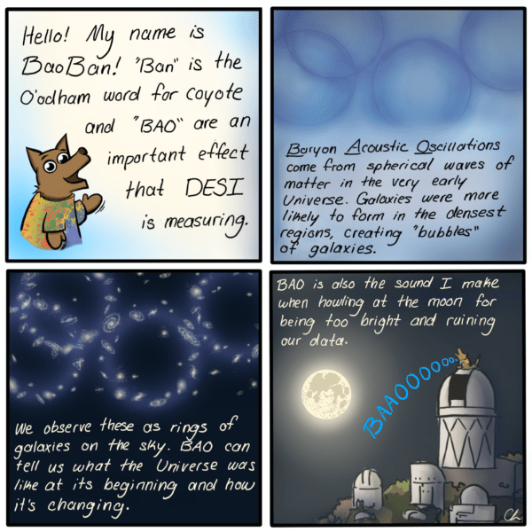
Credit: Claire Lamman

DESI timeline
2015
16
17
18
19
20
22
23
24
21
25
26
27
approved
construction started
first light
comissioning completed
main survey started
Y1 data sample
Y1 results
Y3 data sample secured
end of the survey...
... DESI-2

From images to redshifts


imaging surveys (2014 - 2019) + WISE (IR)
target selection
spectroscopic observations
spectra and redshift measurements

Imaging surveys used by DESI
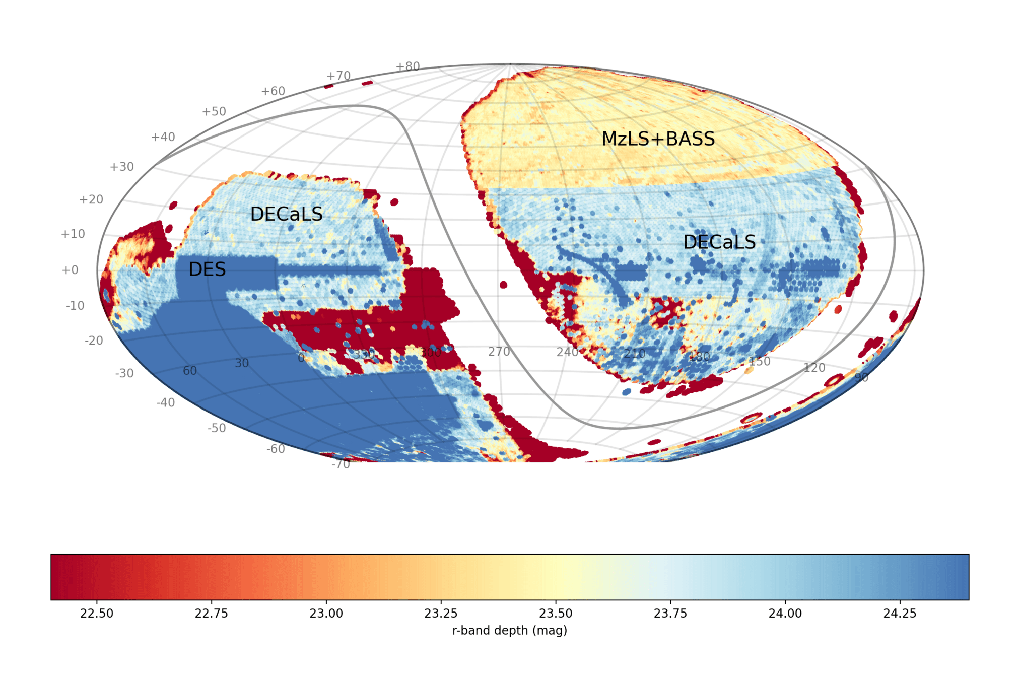

\(\sim 22.7\) in SDSS
\(r\)-band depth
Bok

Imaging surveys used by DESI


\(\sim 23.7\) in North
\(\sim 22.7\) in SDSS
\(r\)-band depth
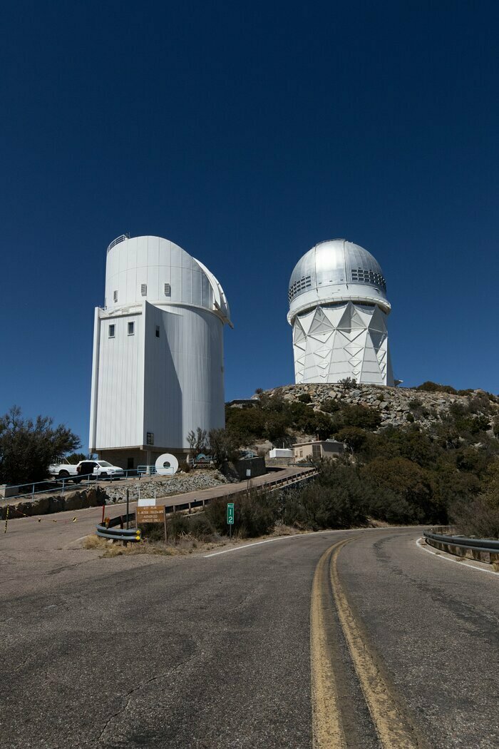
Bok
Mayall
credit: NOIRLab
Optical surveys (grz)
North (5.2k \(\mathrm{deg}^2\))
- BASS (gr): 2016 - 2018
- MzLS (z): 2015 - 2019

Imaging surveys used by DESI


\(\sim 23.7\) in North
\(\sim 22.7\) in SDSS
\(r\)-band depth
Optical surveys (grz)
North (5.2k \(\mathrm{deg}^2\))
- BASS (gr): 2016 - 2018
- MzLS (z): 2015 - 2019
South (11.7k \(\mathrm{deg}^2\))
- DECaLS (grz): 2014 - 2019
\(\sim 24.2\) in South
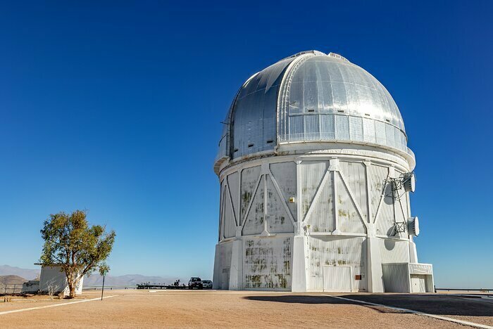
Blanco

Imaging surveys used by DESI
Optical surveys (grz)
North (5.2k \(\mathrm{deg}^2\))
- BASS (gr): 2016 - 2018
- MzLS (z): 2015 - 2019
South (11.7k \(\mathrm{deg}^2\))
- DECaLS (grz): 2014 - 2019
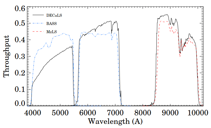

Imaging surveys used by DESI
Infrared survey
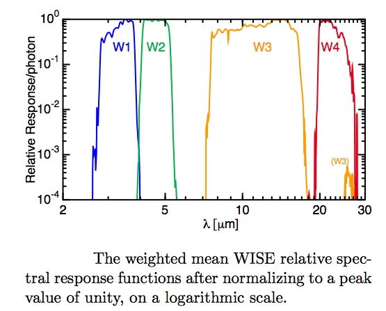
WISE & NEOWISE (W1, W2, W3, W4): 2010 - 2020
Blanco
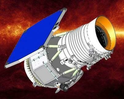

Imaging surveys used by DESI
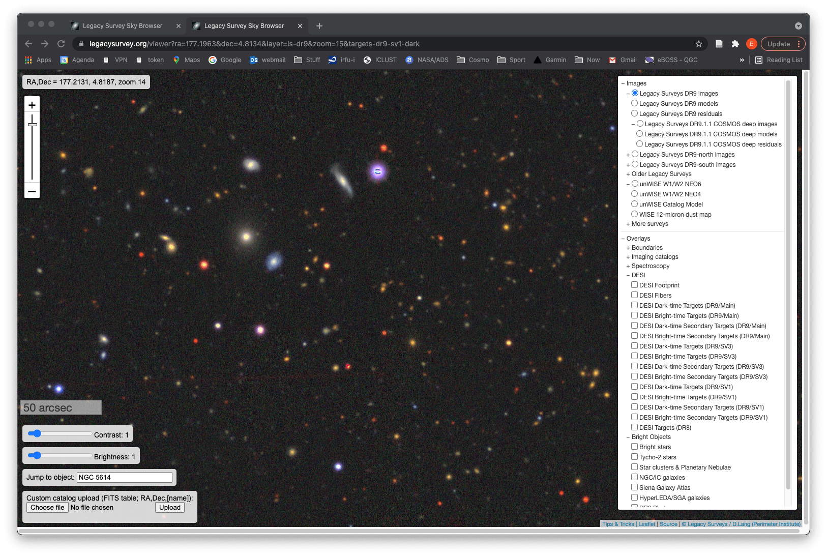
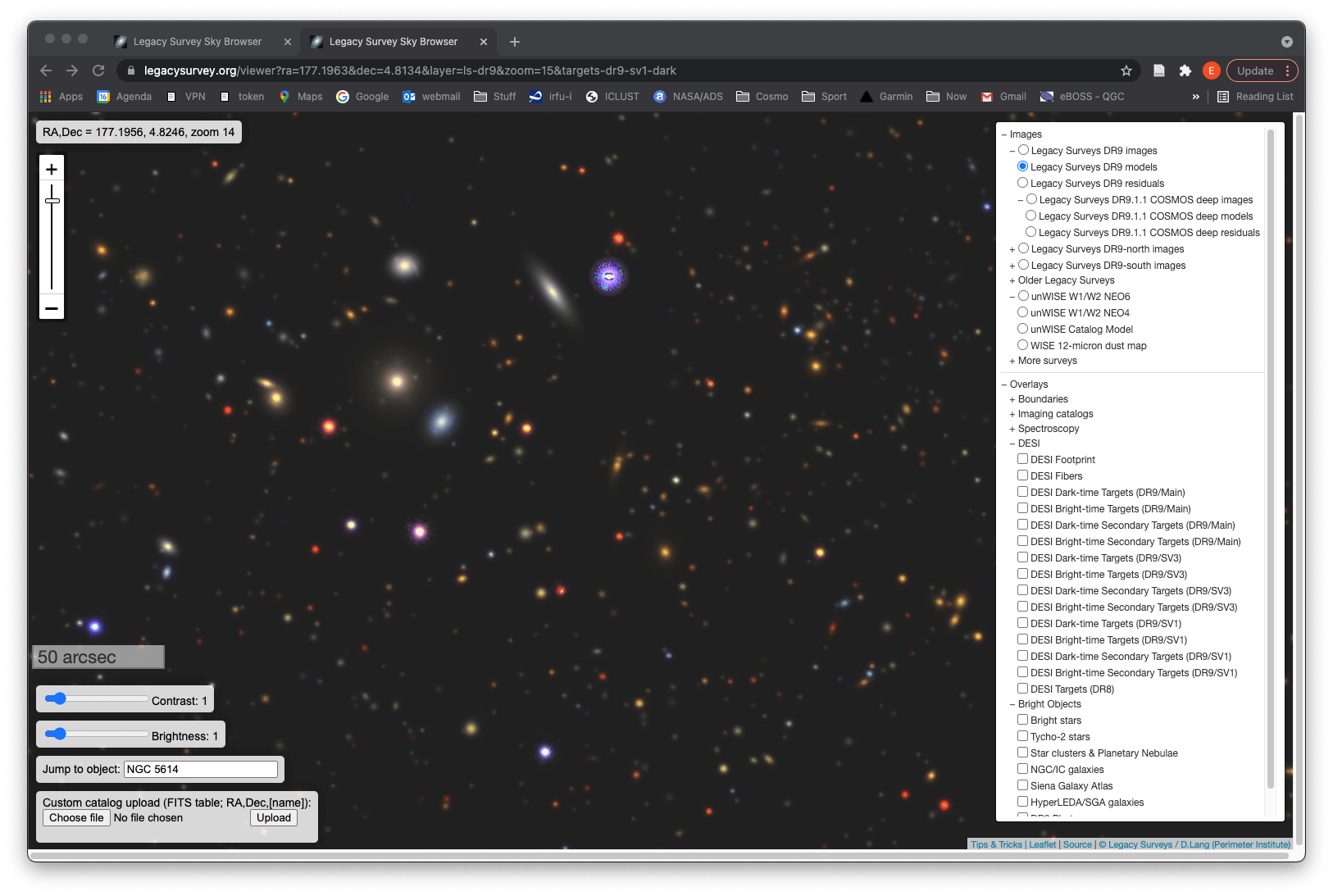
visit legacysurvey.org

Imaging surveys used by DESI

Target selection - BGS (\(0.1 < z < 0.4\))

BGS bright \(\simeq\) 850 targets \(\mathrm{deg}^{-2}\)
BGS faint \(\simeq\) 520 targets \(\mathrm{deg}^{-2}\)
\(19.5 < r < 20.2\)
\(r < 19.5\)

Target selection - LRG (\(0.4 < z < 1.1\))
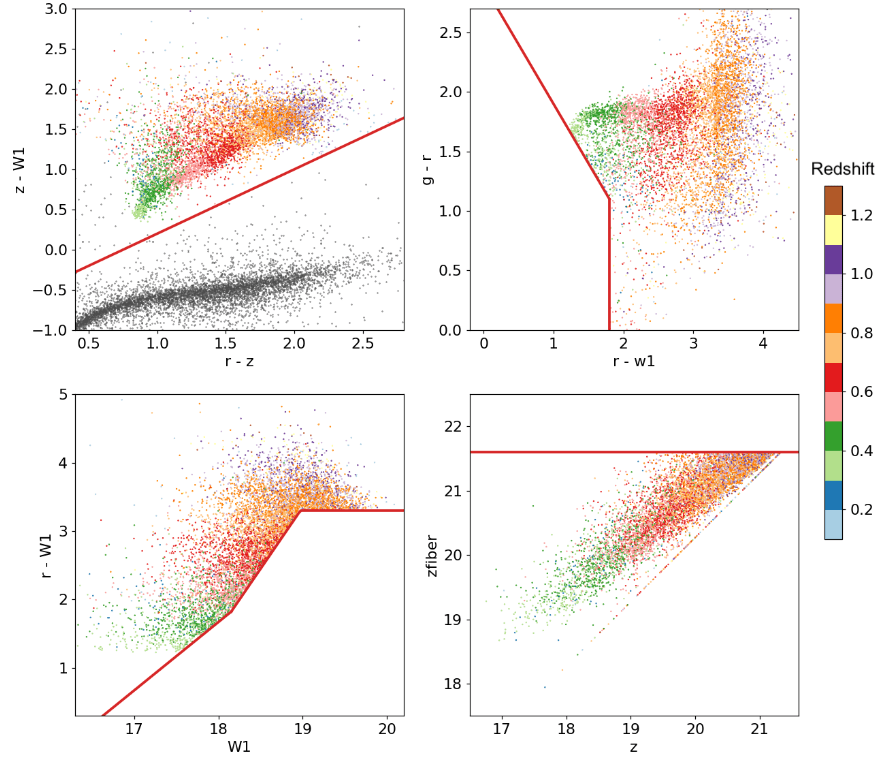
a) star rejection
b) redshift
c) density
d) spectro S/N
\(\simeq\) 640 targets \(\mathrm{deg}^{-2}\)
a) star rejection with WISE
b) \(g - W1 > 2.9\) selects targets with \(z > 0.3\)
c) slope of \(r - W1\) vs \(W1\) chosen to produce ~ constant number density \(0.4 < z < 0.8\)
d) spectro S/N with z-fiber cut

Target selection - ELG (\(0.6 < z < 1.6\))
\(\simeq\) 1940 targets \(\mathrm{deg}^{-2}\)
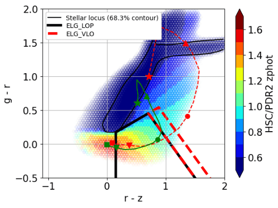
a) number density tuned with \(g\mathrm{fiber} < 24.1\)
b) star / low-\(z\) rejection with \(g - r\) vs \(r - z\)
c) rejection of \(z > 1.6\) with \(g - r\) cut
d) high [OII] with \(g - r\) vs \(r - z\)
c) high-z
b) star / low-z rejection
d) [OII]

Target selection - QSO (\(0.8 < z < 3.5\))
a) PSF-type objects
b) 16.5 < r < 23 cut to remove bright stars, low S/N spectro
c) QSO separated from stars with excess infrared from the dusty torus: W1, W2 > 22.3 and random forest trained on grzW1W2 colors
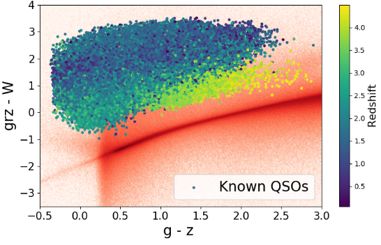
stellar locus
\(\simeq\) 310 targets \(\mathrm{deg}^{-2}\)

Target selection
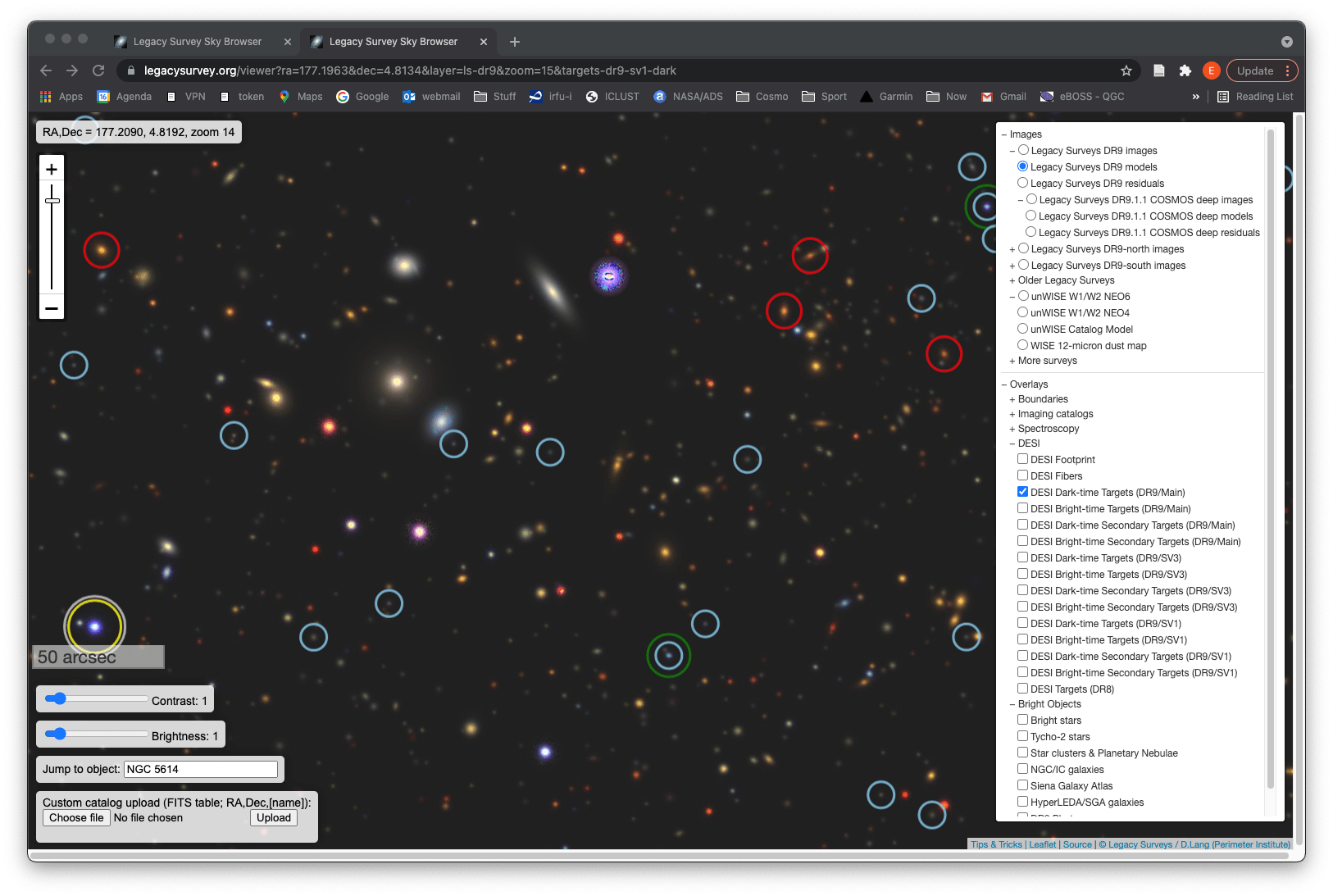

Target selection
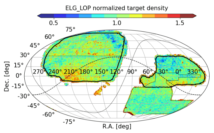


From images to redshifts


imaging surveys (2014 - 2019) + WISE (IR)
target selection
spectroscopic observations
spectra and redshift measurements

Mayall Telescope
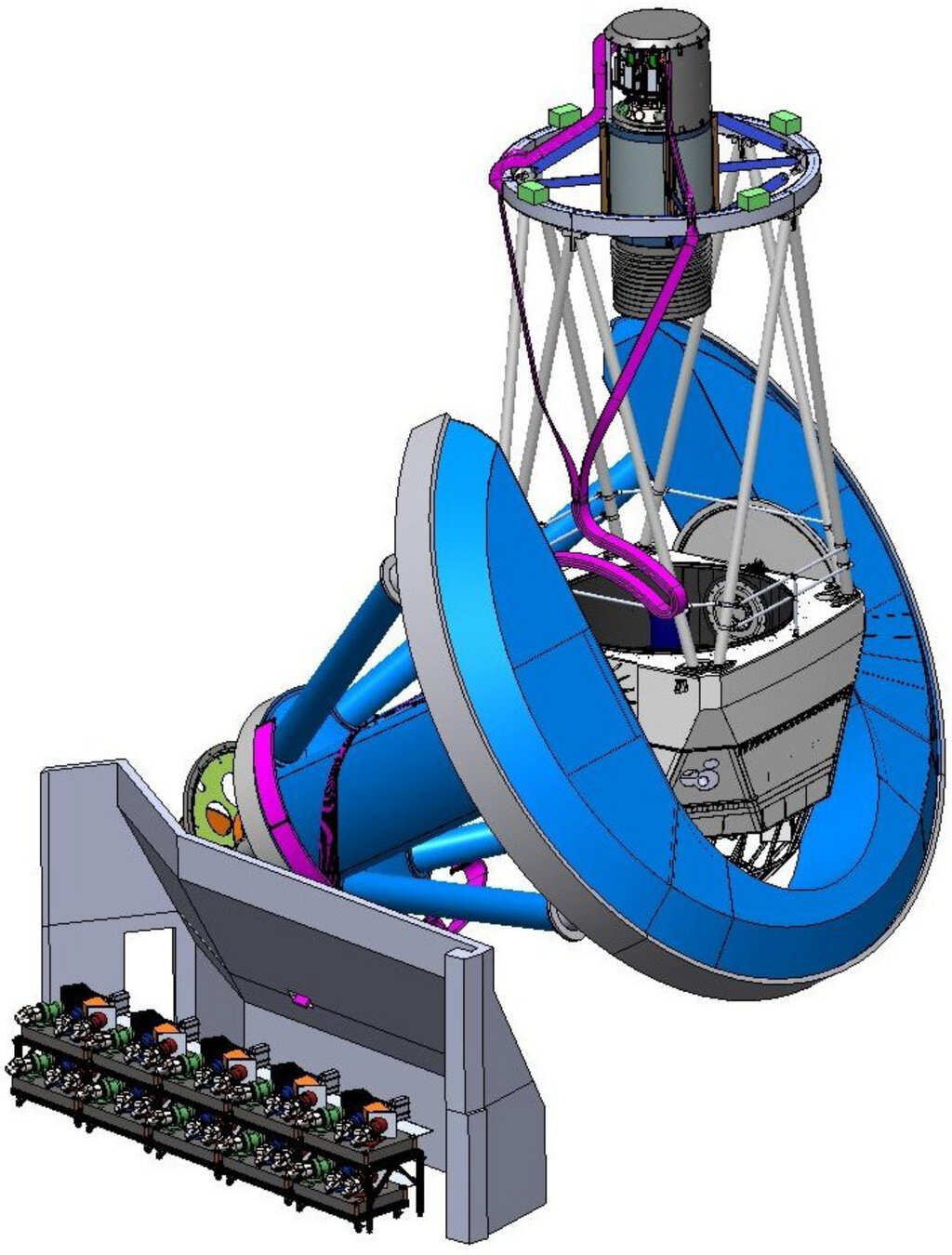
focal plane 5000 fibers
wide-field corrector
6 lenses, FoV \(\sim 8~\mathrm{deg}^{2}\)
Kitt Peak, AZ
4 m mirror

Mayall Telescope

focal plane 5000 fibers
fiber view camera
ten 3-channel spectrographs
49 m, 10-cable fiber run
Kitt Peak, AZ


Mayall Telescope
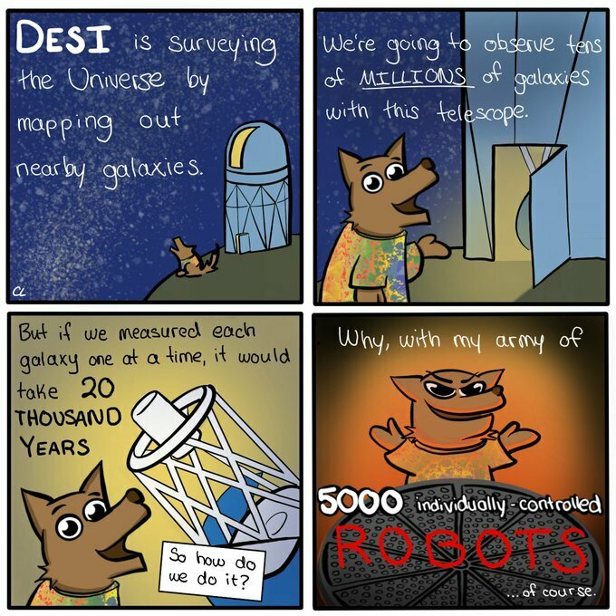

Credit: Claire Lamman
For more BaoBan adventures, see cmlamman.github.io/baoban_comics.html

Focal plane: 5000 robotic positioners
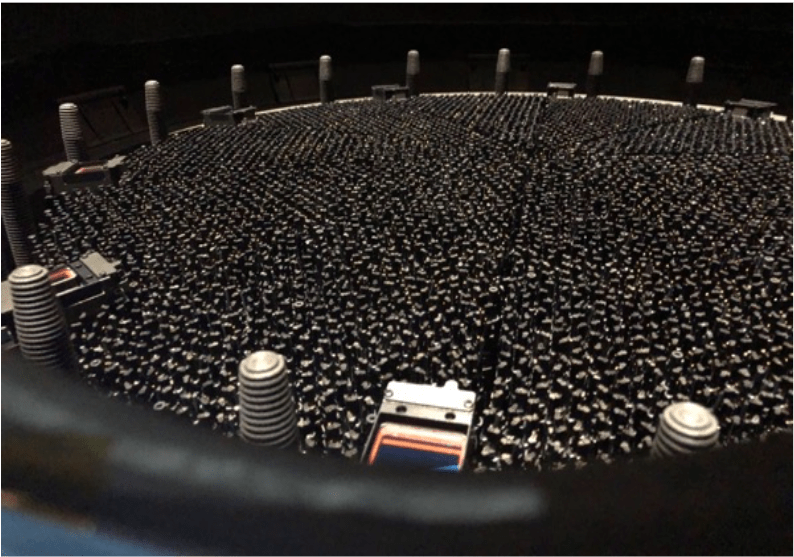
86 cm
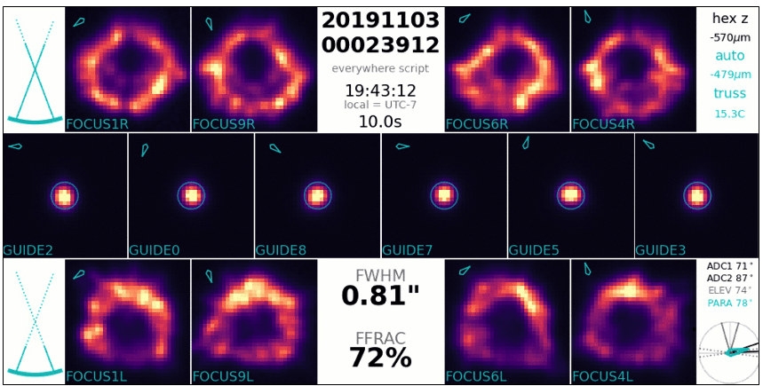
GFA: Guide/Focus/Alignment

Focal plane: 5000 robotic positioners


Focal plane: 5000 robotic positioners

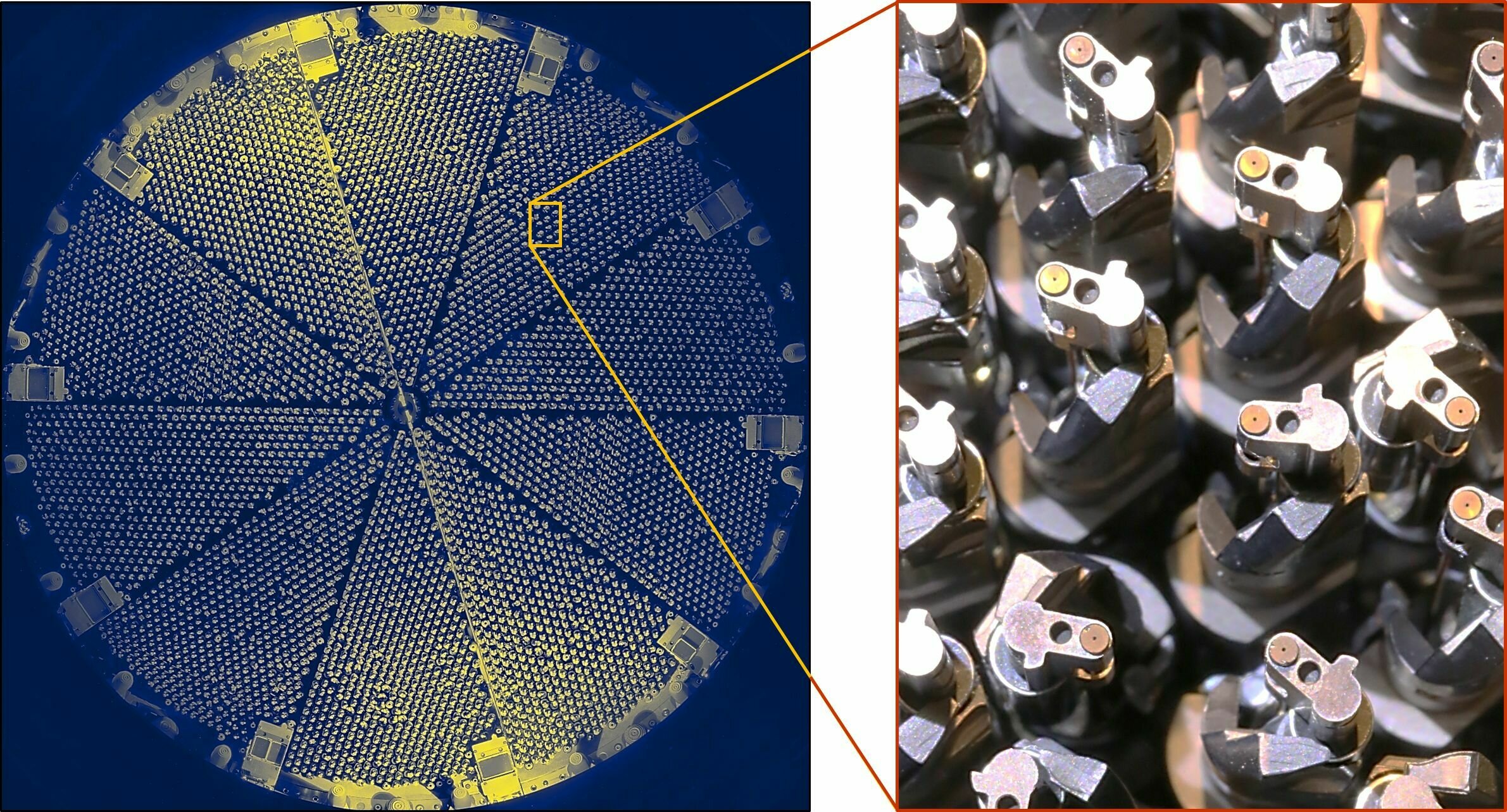


Robotic positioner
= 1.4 arcsec (~seeing)
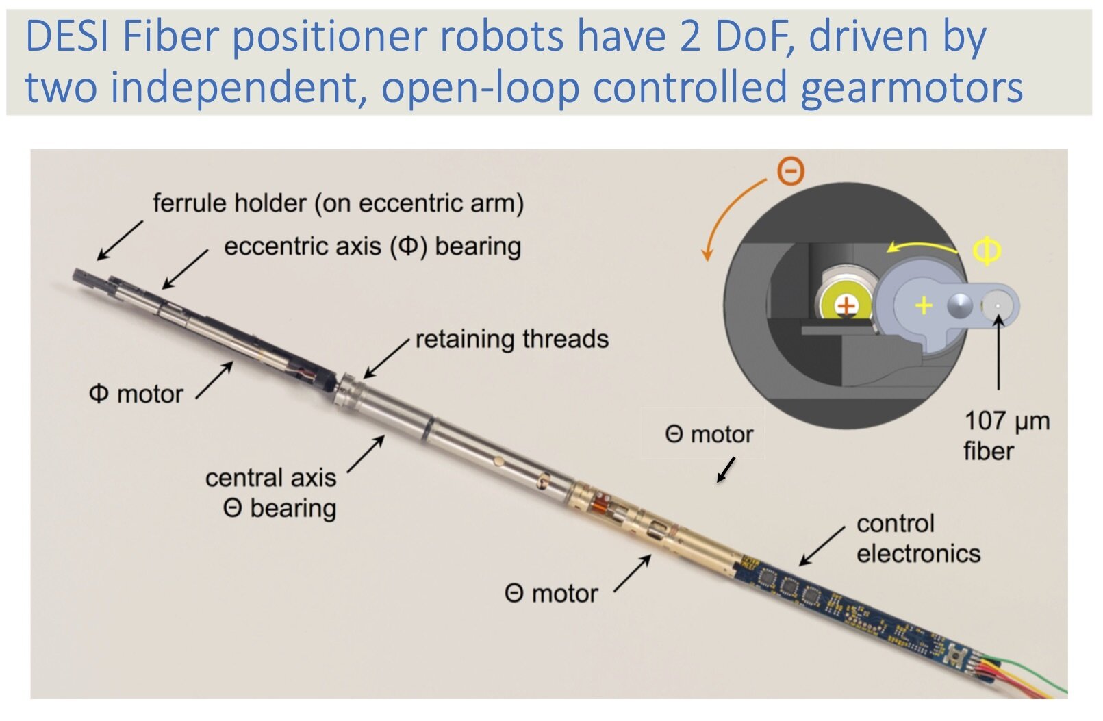
2 DoF \((\Theta, \Phi)\): 2 motors in open-loop

Fiber view camera
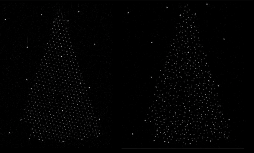
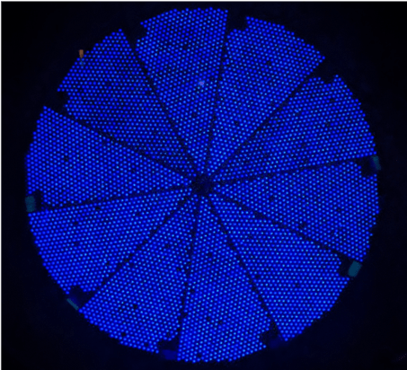
fibers illuminated from spectrographs
FVC takes image through the corrector
positioning: "blind" move (50\(\mu\mathrm{m}\)), "correction" move (6\(\mu\mathrm{m}\))
"Fiber collisions"

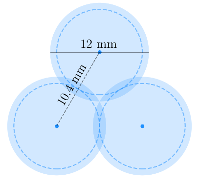
Groups of galaxies too close to each other cannot all receive a fiber
\(0.05^\circ \simeq\) positioner patrol diameter

Observing sequence
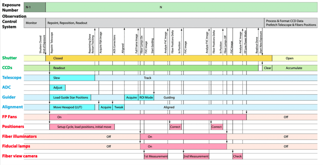
Reposition & readout in <2min!
Exposure time (dark) 1000 s

Spectrographs
fibers illuminated from spectrographs
FVC takes image through the corrector
positioning

10 identical 500 fiber spectrographs
3 arms (red, blue, NIR)
Linear Pulse Tube cooled
French technical contribution
(CEA, CNRS)
Vendor (French!)

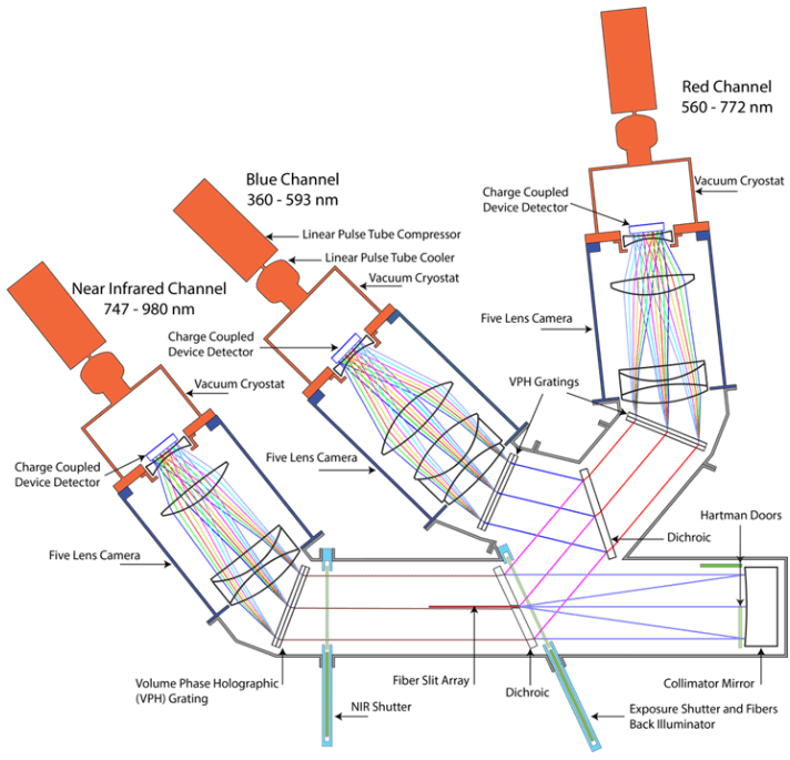

Spectroscopic pipeline

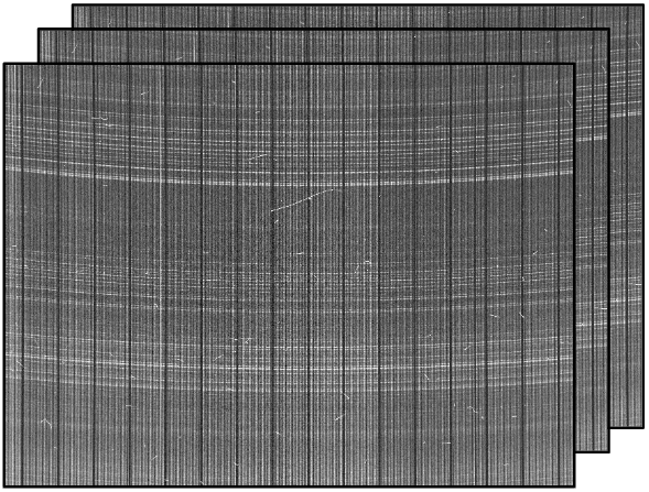
wavelength
fiber number
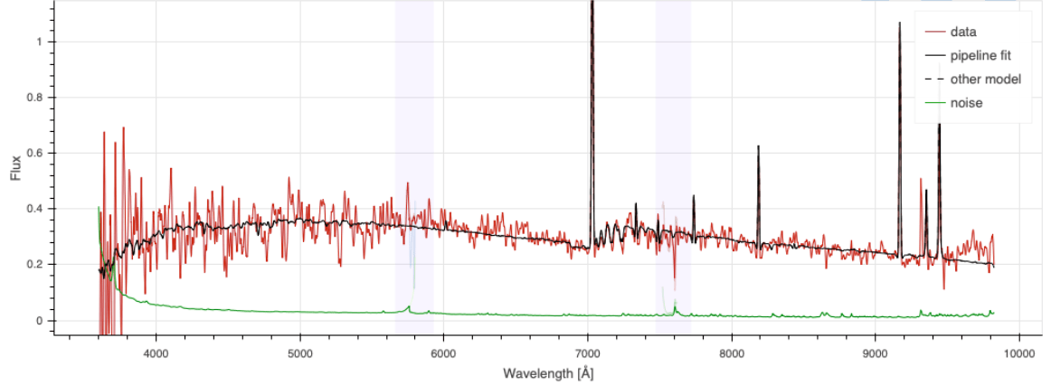

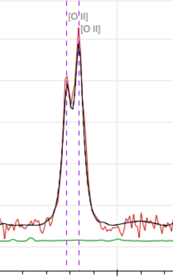
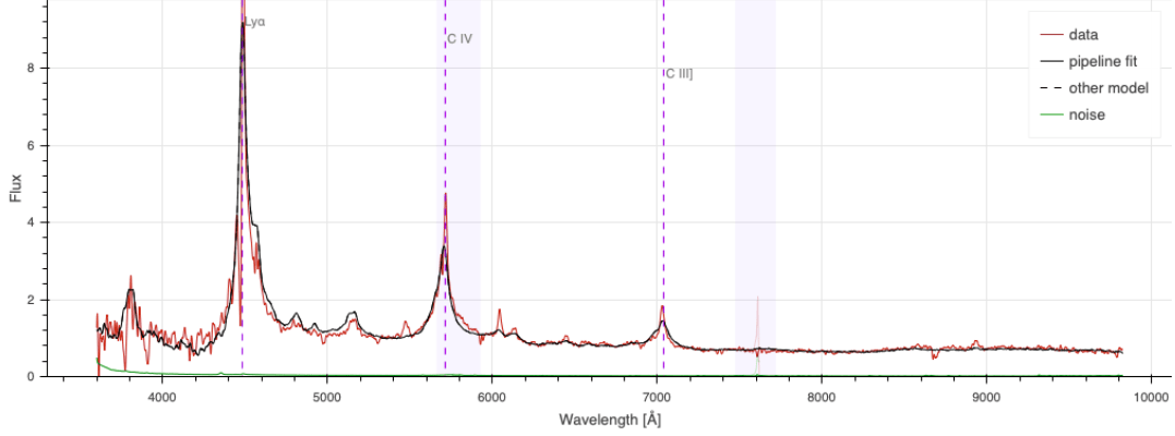
\(z = 2.1\) QSO
\(z = 0.9\) ELG
Ly\(\alpha\)
CIV
CIII
[OII] doublet at \(2727 \AA\) up to \(z = 1.6\)
[OII]
Ly\(\alpha\) at \(1216 \AA\) down to \(z = 2.0\)

Survey strategy
Full Survey: 14,000 \(\mathrm{deg}^{2}\)
Field of view: 8 \(\mathrm{deg}^{2}\) \(\simeq\) 42 full moon

dark time: LRG, ELG, QSO - 7 passes bright time: BGS - 4 passes
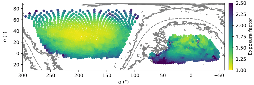

Survey strategy
Full Survey: 14,000 \(\mathrm{deg}^{2}\)
| asgn. comp. (Y5) | z. comp. | #good z (Y5) | |
| BGS | 80% | 99% | 13.8M |
| LRG | 90% | 99% | 7.5M |
| ELG | 60% | 73% | 15.7M |
| QSO | 99% | 67% | 2.9M |
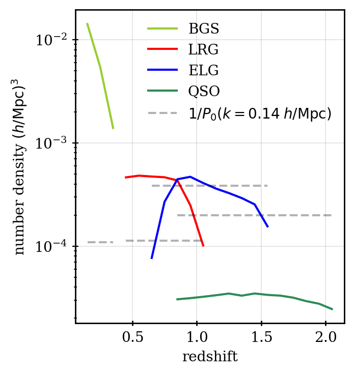

DESI data release 1 (DR1)
Observations from May 14th 2021 to June 12th 2022


DESI data release 1 (DR1)
Observations from May 14th 2021 to June 12th 2022

| asgn. comp. | Y1 / Y5 | |
| BGS | 64% | 40% |
| LRG | 69% | 30% |
| ELG | 35% | 21% |
| QSO | 87% | 50% |

The Contreras Fire (June 11 - 17 2022)
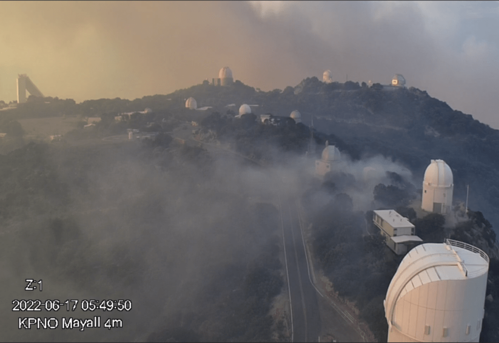

The Contreras Fire (June 11 - 17 2022)

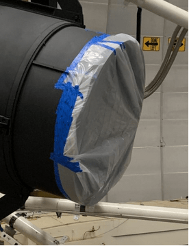
Credit: Bob Stupak

The Contreras Fire (June 11 - 17 2022)
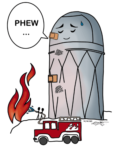
Credit: Clara Delabrouille

DESI data release 1 (DR1)


5.7 million unique redshifts at z < 2.1 and > 420,000 Ly\(\alpha\) QSO at z > 2.1

Release of DESI Y1 (BAO) results
April 4th 2024
First batch of DESI Y1 cosmological analyses
data.desi.lbl.gov/doc/papers/
• DESI 2024 I: First year data release
• DESI 2024 II: DR1 catalogs
• DESI 2024 III: BAO from Galaxies and Quasars
• DESI 2024 IV: BAO from the Lyman-Forest
• DESI 2024 V: RSD from Galaxies and Quasars
• DESI 2024 VI: Cosmological constraints from BAO measurements
• DESI 2024 VII: Cosmological constraints from RSD measurements

Correlation functions


Correlation functions


BAO peak

Power spectra


Power spectra


BAO wiggles

Some fits: configuration space

isotropic measurement
anisotropic measurement

Some fits: Fourier space

isotropic measurement
anisotropic measurement

Non-linear evolution
Non-linear structure growth and peculiar velocities blur and shrink (slightly) the ruler


Eisenstein et al. 2008, Padmanabhan et al. 2012

Density field reconstruction
Estimates Zeldovich displacements from observed field and moves galaxies back: refurbishes the ruler (improves precision and accuracy)


reconstruction

Density field reconstruction


DESI Y1 BAO analysis
- Biggest ever spectroscopic BAO dataset (\(N_\mathrm{tracer}\) and \(V\))

5.7 million unique redshifts
Effective volume \(V_\mathrm{eff} = 18 \; \mathrm{Gpc}^{3}\)
\(3 \times \) bigger than SDSS!

DESI Y1 BAO analysis
- Biggest ever spectroscopic BAO dataset (\(N_\mathrm{tracer}\) and \(V\))
- Blind analysis to mitigate observer / confirmation biases (catalog-level blinding)
fiducial cosmology
blinded cosmology (\(\Omega_\mathrm{m}, w_0, w_a\))
(random & unknown)

DESI Y1 BAO analysis
- Biggest ever spectroscopic BAO dataset (\(N_\mathrm{tracer}\) and \(V\))
- Blind analysis to mitigate observer / confirmation biases (catalog-level blinding)
fiducial cosmology
blinded cosmology (\(\Omega_\mathrm{m}, w_0, w_a\))
(random & unknown)
+ RSD blinding: change reconstructed peculiar velocities
+ \(f_\mathrm{NL}\) blinding: add clustering-dependent signal on large scales with weights

DESI Y1 BAO analysis
- Biggest ever spectroscopic BAO dataset (\(N_\mathrm{tracer}\) and \(V\))
- Blind analysis to mitigate observer / confirmation biases (catalog-level blinding)
- Theory developments in BAO fitting code


DESI Y1 BAO analysis
- Biggest ever spectroscopic BAO dataset (\(N_\mathrm{tracer}\) and \(V\))
- Blind analysis to mitigate observer / confirmation biases (catalog-level blinding)
- Theory developments in BAO fitting code
- New and improved reconstruction methods
- New combined tracer method used for overlapping galaxy samples (LRG and ELG in \(0.8 < z < 1.1\))
- Unified BAO pipeline applied to all (discrete) tracer / redshift bins consistently

Tests of systematic errors
Considered many possible sources of systematic errors using simulations and data:
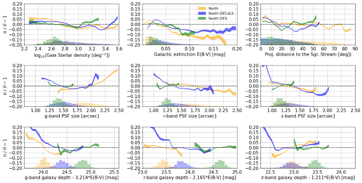
- observational effects (imaging systematics, fiber collisions)
- BAO reconstruction (2 algorithms compared)
- covariance matrix construction
- incomplete theory modelling
- choice of fiducial cosmology
- galaxy-halo (HOD) model uncertainties
no systematics detected
systematics << statistics
Max effect: \(\sigma_\mathrm{stat. + syst.} < 1.05 \sigma_\mathrm{stat.}\)

Release of DESI Y1 (BAO) results
April 4th 2024
First batch of DESI Y1 cosmological analyses
https://data.desi.lbl.gov/doc/papers/
• DESI 2024 I: First year data release
• DESI 2024 II: DR1 catalogs
• DESI 2024 III: BAO from Galaxies and Quasars
• DESI 2024 IV: BAO from the Lyman-Forest
• DESI 2024 V: RSD from Galaxies and Quasars
• DESI 2024 VI: Cosmological constraints from BAO measurements
• DESI 2024 VII: Cosmological constraints from RSD measurements

Ly\(\alpha\) forest
Absorption in QSO spectra by neutral hydrogen in the intergalactic medium: \(\lambda_\mathrm{abs} = (1 + z_\mathrm{HI}) \times 1215.17 \; \AA \)
Transmitted flux fraction \(F = e^{-\tau}\) probes the fluctuation in neutral hydrogen density, \(\tau \propto n_\mathrm{HI} \)
credit: Andrew Pontzen

Ly\(\alpha\) correlation functions in DESI Y1


Ly\(\alpha\) - Ly\(\alpha\)
Ly\(\alpha\) - QSO
QSO
QSO
HI cloud
HI cloud
HI cloud
QSO


DESI Y1 Ly\(\alpha\) BAO analysis
- Biggest ever Ly\(\alpha\) dataset (\(N_\mathrm{tracer}\))
>420,000 Ly\(\alpha\) QSO at z > 2.1
\(2 \times \) more than SDSS!


DESI Y1 Ly\(\alpha\) BAO analysis
- Biggest ever Ly\(\alpha\) dataset (\(N_\mathrm{tracer}\))
- First blind analysis to mitigate observer / confirmation biases (correlation function-level blinding)

DESI Y1 Ly\(\alpha\) BAO analysis
- Biggest ever Ly\(\alpha\) dataset (\(N_\mathrm{tracer}\))
- First blind analysis to mitigate observer / confirmation biases (correlation function-level blinding)
- Modelling of the correlation function: cosmological signal, and many contaminants!

DESI Y1 Ly\(\alpha\) BAO analysis
- Biggest ever Ly\(\alpha\) dataset (\(N_\mathrm{tracer}\))
- First blind analysis to mitigate observer / confirmation biases (correlation function-level blinding)
- Modelling of the correlation function: cosmological signal, and many contaminants!
- Very stable results, systematic uncertainty neglected

Release of DESI Y1 (BAO) results
April 4th 2024
First batch of DESI DR1 cosmological analyses
https://data.desi.lbl.gov/doc/papers/
• DESI 2024 I: First year data release
• DESI 2024 II: DR1 catalogs
• DESI 2024 III: BAO from Galaxies and Quasars
• DESI 2024 IV: BAO from the Lyman-Forest
• DESI 2024 V: RSD from Galaxies and Quasars
• DESI 2024 VI: Cosmological constraints from BAO measurements
• DESI 2024 VII: Cosmological constraints from RSD measurements

- transverse to the line-of-sight: \(D_\mathrm{M}(z) / r_\mathrm{d}\)
- along the line-of-sight: \(D_\mathrm{H}(z) / r_\mathrm{d} = c / (H(z) r_\mathrm{d}) \)
- low S/N, isotropic average: \( D_\mathrm{V}(z) / r_\mathrm{d} = (z D_{\mathrm{M}}^{2}(z) D_\mathrm{H}(z))^{1/3} / r_\mathrm{d}\)
BAO measurements
BAO measures ratios of distances over the sound horizon scale at the drag epoch ["standard ruler"] \(r_\mathrm{d}\)

Let's factor out the \(h\) terms:
- \(\color{blue}{[D_\mathrm{M}(z) h] (\Omega_\mathrm{m}, f_\mathrm{DE}, \Omega_\mathrm{K}, ...)} \color{black}{/} \color{orange}{[r_\mathrm{d}(\Omega_\mathrm{m} h^{2}, \Omega_\mathrm{b} h^{2}) h]} \)
- \( \color{blue}{[D_\mathrm{H}(z) h] (\Omega_\mathrm{m}, f_\mathrm{DE}, \Omega_\mathrm{K}, ...)} \color{black}{/} \color{orange}{[r_\mathrm{d}(\Omega_\mathrm{m} h^{2}, \Omega_\mathrm{b} h^{2}) h]} \)
BAO measurements at different \(z\) constrain:
- energy content \( \color{blue}{(\Omega_\mathrm{m}, f_\mathrm{DE}, ...)} \)
- constant-over-\(z\) product \(\color{orange}{r_\mathrm{d} h}\) i.e. \(\color{orange}{H_{0} r_\mathrm{d}}\)
These quantities directly relate to base cosmological parameters
BAO measurements
\(h = H_{0} / [100\; \mathrm{km}/\mathrm{s} / \mathrm{Mpc}]\)
\(\Omega_\mathrm{m}\) fractional energy density of matter
\(f_\mathrm{DE}\) dark energy
\(\Omega_\mathrm{K}\) curvature
\(\Omega_{b}\) baryons


DESI Y1 BAO

DESI BAO measurements


DESI Y1 BAO

DESI BAO measurements


DESI Y1 BAO

DESI BAO measurements


DESI Y1 BAO

DESI BAO measurements


DESI Y1 BAO

DESI BAO measurements


DESI Y1 BAO

DESI BAO measurements

DESI Y1 BAO

DESI BAO measurements
Consistent with each other,
and complementary
Consistency with other probes

DESI Y1 BAO consistent with:

Consistency with other probes

DESI Y1 BAO consistent with:

Consistency with other probes

DESI Y1 BAO consistent with:
- SDSS eBOSS Collaboration, 2020
- primary CMB: Planck Collaboration, 2018 and CMB lensing: Planck PR4 + ACT DR6 lensing ACT Collaboration, 2023, Carron, Mirmelstein, Lewis, 2022

Consistency with other probes

DESI Y1 BAO consistent with:
- SDSS eBOSS Collaboration, 2020
- primary CMB: Planck Collaboration, 2018 and CMB lensing: Planck PR4 + ACT DR6 lensing ACT Collaboration, 2023, Carron, Mirmelstein, Lewis, 2022


- BAO constrains \( r_\mathrm{d}(\blue{\Omega_\mathrm{m}} h^{2}, \orange{\Omega_\mathrm{b} h^{2}}) h \)
- \( \blue{\Omega_\mathrm{m}} \) constrained by BAO at different \(z\)
- \(\orange{\Omega_\mathrm{b}h^2}\) can be constrained by light element abundance from Big Bang Nucleosynthesis (BBN): Schöneberg et al., 2024
\(\implies\) constraints on \(h\) i.e. \(H_0 = 100 h \; \mathrm{km} / \mathrm{s} / \mathrm{Mpc}\)
Hubble constant

Hubble constant
\(\theta_\ast\) CMB angular acoustic scale


- Consistency with SDSS
Hubble constant


- Consistency with SDSS
- In agreement with CMB
Hubble constant


- Consistency with SDSS
- In agreement with CMB
- In \(3.7 \sigma\) tension with SH0ES
Hubble constant


DESI + CMB measurements favor a flat Universe

Spatial curvature
Dark Energy Equation of State

Dark Energy fluid, pressure \(p\), density \(\rho\)
Equation of State parameter \(w = p / \rho\)
Linked to the evolution of Dark Energy \(w(z) = -1 + \frac{1}{3}\frac{d \ln f_\mathrm{DE}(z)}{d \ln (1 + z)}\)
Dark Energy Equation of State


Constant EoS parameter \(w = p / \rho\)
Dark Energy Equation of State


Constant EoS parameter \(w = p / \rho\)
Dark Energy Equation of State


SNe:
- Pantheon+ Brout, Scolnic, Popovic et al., 2022
Constant EoS parameter \(w = p / \rho\)
Dark Energy Equation of State


SNe:
- Pantheon+ Brout, Scolnic, Popovic et al., 2022
- Union3 Rubin, Aldering, Betoule et al. 2023
Constant EoS parameter \(w = p / \rho\)
Dark Energy Equation of State

SNe:
- Pantheon+ Brout, Scolnic, Popovic et al., 2022
- Union3 Rubin, Aldering, Betoule et al. 2023
- DES-SN5YR DES Collaboration et al. 2024

Constant EoS parameter \(w = p / \rho\)
Dark Energy Equation of State

Assuming a constant EoS, DESI BAO fully compatible with a cosmological constant...

Constant EoS parameter \(w = p / \rho\)

Dark Energy Equation of State

Varying EoS

Dark Energy Equation of State

Varying EoS

Dark Energy Equation of State

Varying EoS

Dark Energy Equation of State

Varying EoS

Dark Energy Equation of State

Varying EoS

Dark Energy Equation of State
Combining all DESI + CMB + SN


Dark Energy Equation of State
Combining all DESI + CMB + SN


Dark Energy Equation of State
Combining all DESI + CMB + SN


Dark Energy Equation of State
Combining all DESI + CMB + SN
\(w_{0} > -1, w_{a} < 0\) favored, level varying on the SN dataset

Sum of neutrino masses

Internal CMB degeneracies limiting precision on the sum of neutrino masses

Sum of neutrino masses

Internal CMB degeneracies limiting precision on the sum of neutrino masses
Broken by BAO, especially through \(H_{0}\)
Low preferred value of \(H_{0}\) yields
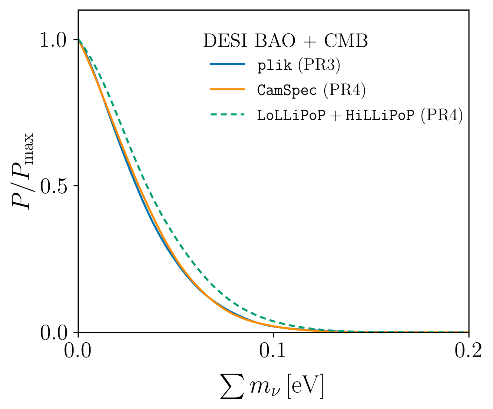
\(\sum m_\nu < 0.072 \, \mathrm{eV} \; (95\%, \color{green}{\text{DESI + CMB})}\)

Limit relaxed for extensions to \(\Lambda\mathrm{CDM}\)
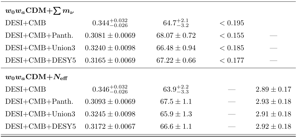
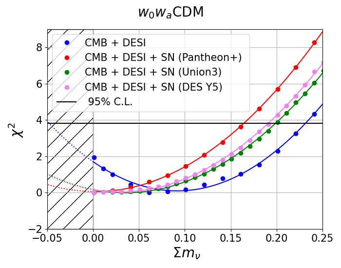
\(\sum m_\nu < 0.195 \, \mathrm{eV}\) for \(w_0w_a\mathrm{CDM}\)
Neutrino mass hierarchies


With \(> 0.059 \, \mathrm{eV}\) prior (NH)
Neutrino mass hierarchies


With \(> 0.059 \, \mathrm{eV}\) prior (NH)
With \(> 0.1 \, \mathrm{eV}\) prior (IH)
Neutrino mass hierarchies


With \(> 0.059 \, \mathrm{eV}\) prior (NH)
With \(> 0.1 \, \mathrm{eV}\) prior (IH)
Current constraints do not strongly favor normal over inverted hierarchy (\(\simeq 2 \sigma\))
Y1 BAO constraints: a summary

DESI already has the most precise BAO measurements ever
Y1 BAO constraints: a summary

DESI already has the most precise BAO measurements ever
DESI BAO is consistent (at the \(\sim 1.9\sigma\) level) with CMB in flat ΛCDM
Y1 BAO constraints: a summary

DESI already has the most precise BAO measurements ever
DESI BAO is consistent (at the \(\sim 1.9\sigma\) level) with CMB in flat ΛCDM
In flat ΛCDM, DESI prefers "small \(\Omega_\mathrm{m}\), large \(H_0\) (though \(3.7\sigma\) away from SH0ES), small \(\sum m_\nu\)"
Y1 BAO constraints: a summary

DESI already has the most precise BAO measurements ever
DESI BAO is consistent (at the \(\sim 1.9\sigma\) level) with CMB in flat ΛCDM
In flat ΛCDM, DESI prefers "small \(\Omega_\mathrm{m}\), large \(H_0\) (though \(3.7\sigma\) away from SH0ES), small \(\sum m_\nu\)"
Some hint of time-varying Dark Energy equation of state especially when combined with supernovae measurements
What I haven't talked about

Y1 supporting papers: BAO and Full Shape theory modelling, covariance matrices, BAO reconstruction, etc., see data.desi.lbl.gov/doc/papers/
DESI EDR data public (including 1%: 140 \(\mathrm{deg}^2\), 1.2M extragalactic redshifts): DESI Collaboration 2023 arXiv:2306.06308
A bunch of science papers: Ly\(\alpha\), small scale clustering (HOD), etc., see: data.desi.lbl.gov/doc/papers/edr/
Conclusions

DESI runs beautifully!
Y1 full shape analysis unblinded, papers at the end of 2024
Many alternative analyses! DE reconstruction, \(H_0\) without BAO, modified gravity, higher order statistics, alternative statistics, etc.
DR1 catalogs to be available next year
Y3 data on disk, BAO analysis starting!
Full shape analysis

observed redshift = Hubble flow and peculiar velocities (RSD = "redshift space distortions")

Full shape also driven by primordial physics (\(\omega_m, \omega_b, n_s, f_{\mathrm{NL}}, ...\))
RSD probes growth of structure \(f\sigma_8\), sensitive to gravity, DE, \(\nu\)

Full shape analysis

Three power spectrum EFT models considered:
- pybird
- velocileptors
- folps

credit: Mark Maus, Hernan Noriega, Yan Lai
Full shape analysis - tests

- maximum fitting scale \(k_\mathrm{max}\)
- galaxy - halo connection, bias parametrization, prior choices
- "ShapeFit" template compression, Brieden 2021
- fiducial cosmology
- covariance matrix
- prior volume effects
Full shape analysis

Prior volume effects
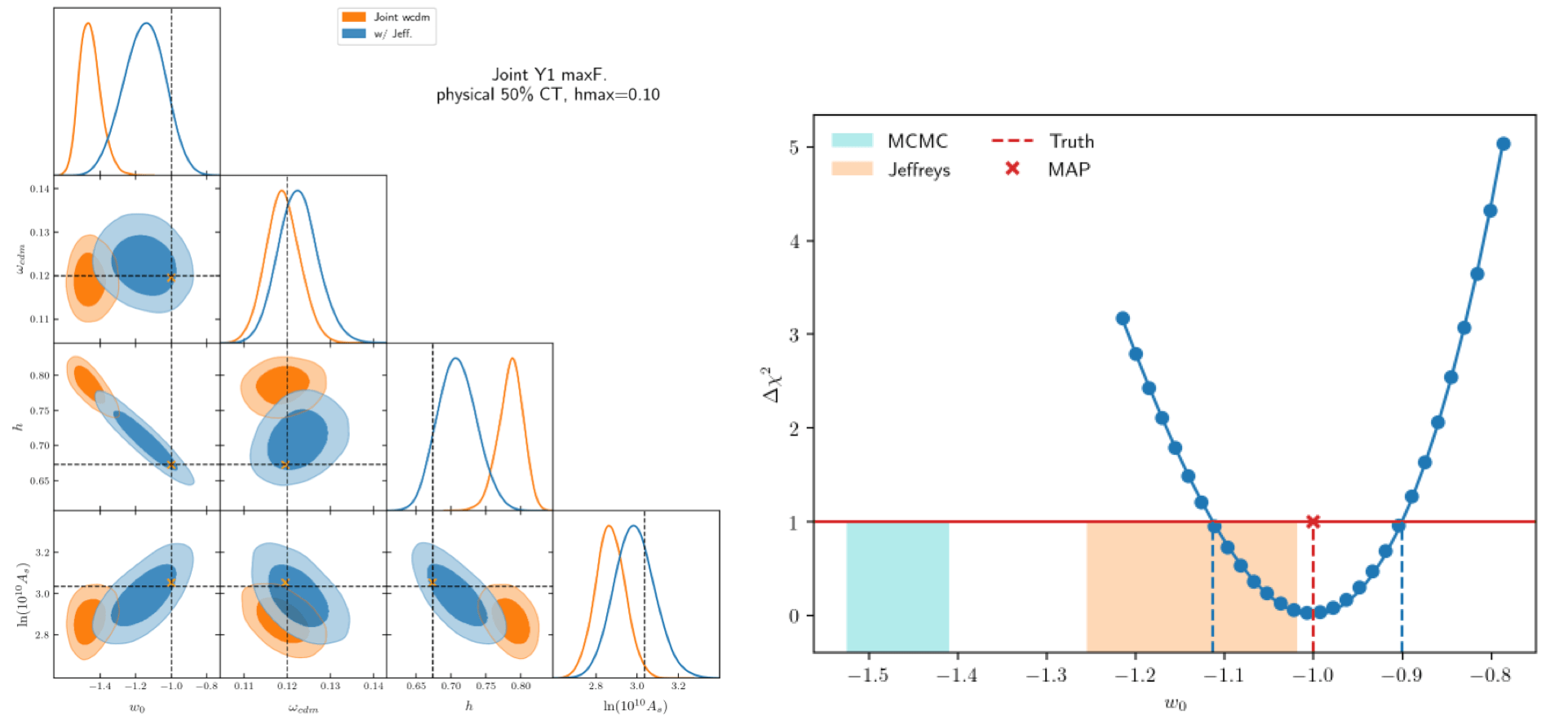
credit: Ruiyang Zhao

Full shape analysis

- \(k_\mathrm{max}\)
- galaxy - halo connection, bias parametrization, prior choices
- "ShapeFit" template compression, Brieden 2021
- fiducial cosmology
- covariance matrix
- prior volume effects
- imaging systematics
- spectroscopic systematics
- "fiber collisions"
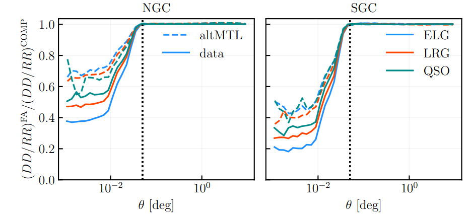
Fiber collisions

Impacts power spectrum measurements (altMTL vs complete)

Fiber collisions

Impacts power spectrum measurements (altMTL vs complete)
Solution: \(\theta\)-cut = remove all pairs \(< 0.05^\circ\), new window matrix

Fiber collisions

New window matrix \(W^\mathrm{cut}\); \(\langle P_o(k) \rangle = W^\mathrm{cut}(k, k^\prime) P_t(k^\prime)\)

Fiber collisions

New window matrix \(W^\mathrm{cut}\); \(\langle P_o(k) \rangle = W^\mathrm{cut}(k, k^\prime) P_t(k^\prime)\)
Very non diagonal: let's "rotate" it


Fiber collisions

Successfully removes the \( > 1 \sigma\) bias

credit: Ruiyang Zhao
Full shape analysis

Tests: stability with \(k_\mathrm{max}\)
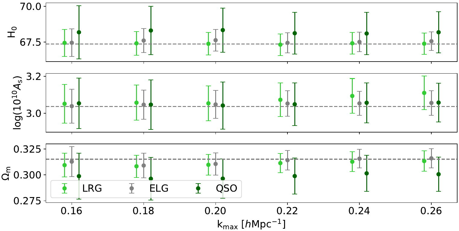
credit: Mark Maus
Full shape analysis

Tests: bias parameterization
- maximal freedom: all 4 bias parameter free
- minimal freedom: \(b_s, b_{3}\) fixed (co-evolution)
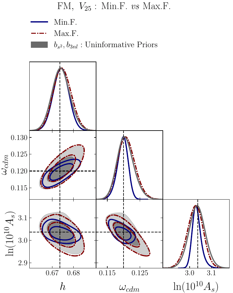
credit: Hernan Noriega

DESI DR1 Ly\(\alpha\) BAO analysis
- Biggest ever Ly\(\alpha\) dataset (\(N_\mathrm{tracer}\))
- First blind analysis to mitigate observer / confirmation biases (correlation function-level blinding)
- Modelling of the correlation function:
- cosmo signal
linear bias + RSD
hydro-sim
BAO

DESI DR1 Ly\(\alpha\) BAO analysis
- Biggest ever Ly\(\alpha\) dataset (\(N_\mathrm{tracer}\))
- First blind analysis to mitigate observer / confirmation biases (correlation function-level blinding)
- Modelling of the correlation function:
- cosmo signal
- high-column density
- metal absorbers
SiII

DESI DR1 Ly\(\alpha\) BAO analysis
- Biggest ever Ly\(\alpha\) dataset (\(N_\mathrm{tracer}\))
- First blind analysis to mitigate observer / confirmation biases (correlation function-level blinding)
- Modelling of the correlation function:
- cosmo signal
- high-column density
- metal absorbers
- correlated noise (sky subtraction)

DESI DR1 Ly\(\alpha\) BAO analysis
- Biggest ever Ly\(\alpha\) dataset (\(N_\mathrm{tracer}\))
- First blind analysis to mitigate observer / confirmation biases (correlation function-level blinding)
- Modelling of the correlation function

physical model fit
+ broadband polynomial

broadband: \(< 0.1\sigma\)

DESI DR1 Ly\(\alpha\) BAO analysis
- Biggest ever Ly\(\alpha\) dataset (\(N_\mathrm{tracer}\))
- First blind analysis to mitigate observer / confirmation biases (correlation function-level blinding)
- Modelling of the correlation function
- Cross-covariance matrix

Correlation matrix
smoothed jackknife, validated with mocks
10% impact on BAO uncertainty

DESI DR1 Ly\(\alpha\) BAO analysis
- Biggest ever Ly\(\alpha\) dataset (\(N_\mathrm{tracer}\))
- First blind analysis to mitigate observer / confirmation biases (correlation function-level blinding)
- Modelling of the correlation function
- Cross-covariance matrix
- Very stable results, systematic uncertainty neglected

Tests of systematic errors


tests with same dataset (not red): shifts \(< \sigma_\mathrm{stat}/3\)
tests with varying datasets (red): shifts consistent with stat.
desilike

- BAO, full shape likelihoods, designed to extend to other observables (lensing, etc.)
- wraps PT codes: velocileptors, pybird, folps(ax)
- automated cobaya / cosmosis / montepython bindings
- wraps samplers, profilers, fisher, in-place emulation
- "JAXification"
template = DirectPowerSpectrumTemplate(z=1.)
theory = LPTVelocileptorsTracerPowerSpectrumMultipoles(ells=(0, 2, 4), template=template)
theory(h=0.7, b1p=1.2)  # returns pk
observable = TracerPowerSpectrumMultipoles(data=data, wmatrix=wmatrix, theory=theory,
										   klim={0: (0.02, 0.2), 2: (0.02, 0.2)})
likelihood = ObservablesGaussianLikelihood(observables=observable)
likelihood(Omega_m=0.3)  # returns log-posterior
Other datasets

- SDSS BAO (for comparisons only): eBOSS Collaboration, 2020
- Primary CMB: Planck Collaboration, 2018
- CMB lensing: Planck PR4 + ACT DR6 lensing ACT Collaboration, 2023, Carron, Mirmelstein, Lewis, 2022
- BBN: Schöneberg et al., 2024
- SN: Pantheon+ Brout, Scolnic, Popovic et al., 2022, Union3 Rubin, Aldering, Betoule et al. 2023, DES-SN5YR DES Collaboration

\(\sum m_\nu\)

credit: Christophe Yèche

\(\sum m_\nu\)
credit: Christophe Yèche
\(w(z)\)


DESI - SDSS consistency (\(\Omega_\mathrm{m}\))


Perfectly consistent!
Using these 2 points alone moves \(\Omega_\mathrm{m}\) by \(< 2 \sigma\)
Are SN \(\Omega_\mathrm{m}\) consistent?


Not so much in flat \(\Lambda\mathrm{CDM}\)...
(so we do not combine them in this model!)
Are SN \(\Omega_\mathrm{m}\) consistent?


Consistent in \(w_0w_a\mathrm{CDM}\)!
plik (PR3) vs PR4 Planck likelihoods

Appendix B
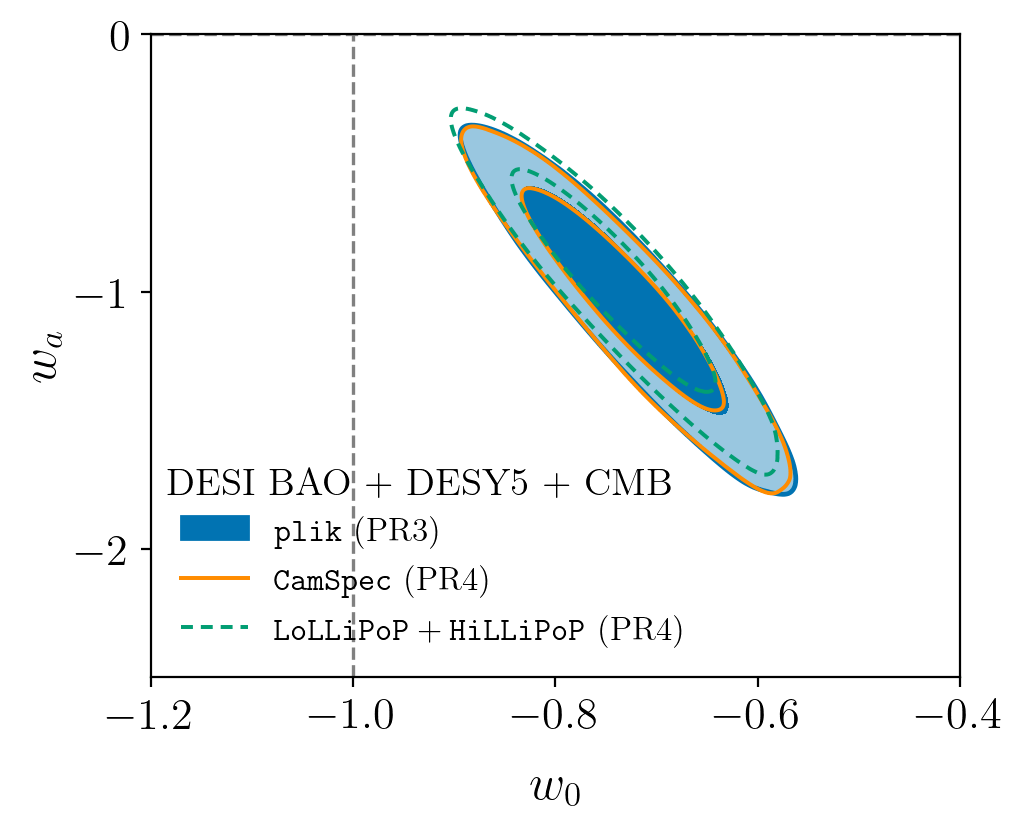
\(w_0 - w_a\) with \(\sum m_\nu\) free


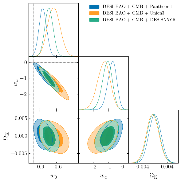
\(w_0 - w_a\) with \(\Omega_\mathrm{K}\)
Preference for \(w_{0} > -1, w_{a} < 0\) persists when curvature is left free
DE constraints driven by low-\(z\) ?

Not that much!
DESI + SDSS swaps DESI measurements with SDSS for \(z < 0.6\)
\(- 0.4 \sigma\) compared to DESI only

\(w(z)\)


Dark energy equation of state:
\(P = w \rho\)
- \(w\) = constant

BAO measurements: dark energy


BAO measurements: dark energy
Full tables

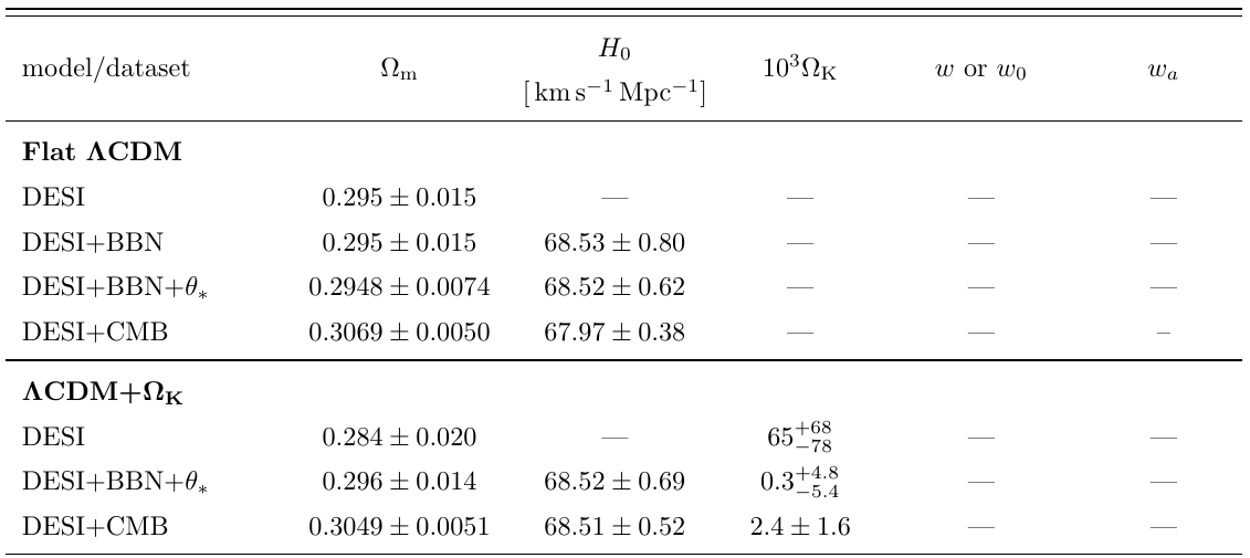
Full tables

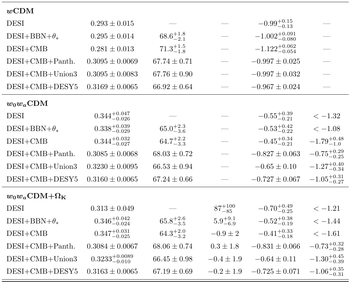

Full tables

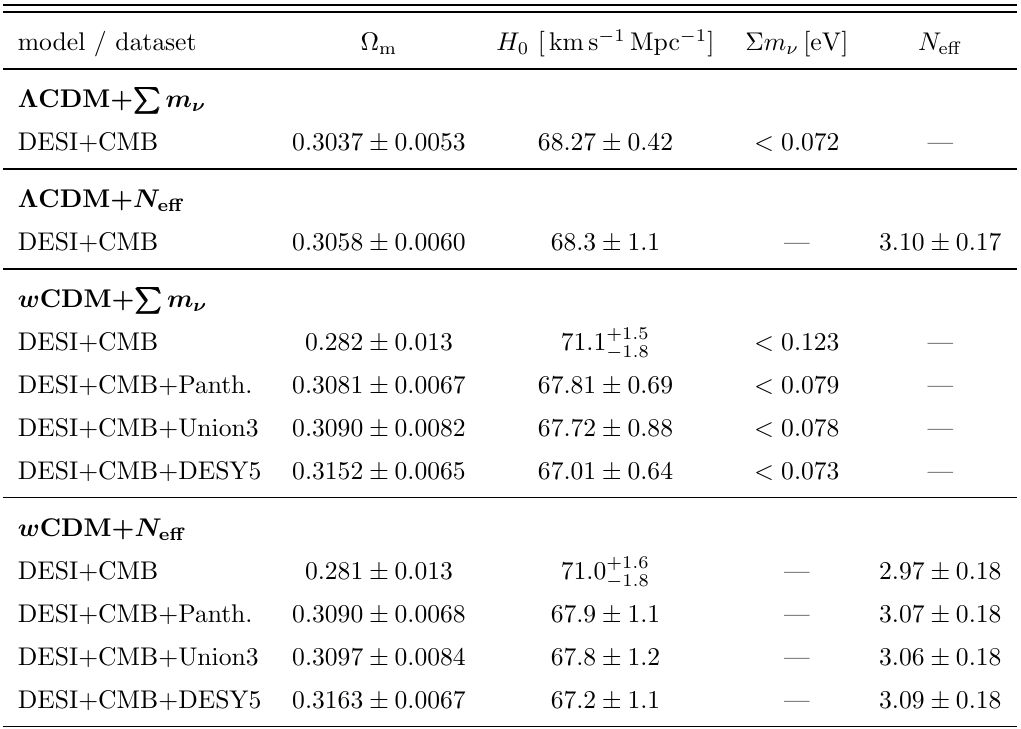
Full tables
