Introduction to galaxy clustering
Arnaud de Mattia
CEA Saclay, Irfu/DPhP
Goals
- broad overview of the domain
- keys to easily read and criticize clustering analysis papers
- to get a bit deeper: Percival 2013, Percival 2018
- History
- Observables and cosmological information
- Spectroscopic surveys and systematics
- Standard (RSD and BAO) analyses
- Current constraints
- On-going and future surveys
- Other clustering analyses
Goals
- broad overview of the domain
- keys to easily read and criticize clustering analysis papers
- to get a bit deeper: Percival 2013, Percival 2018
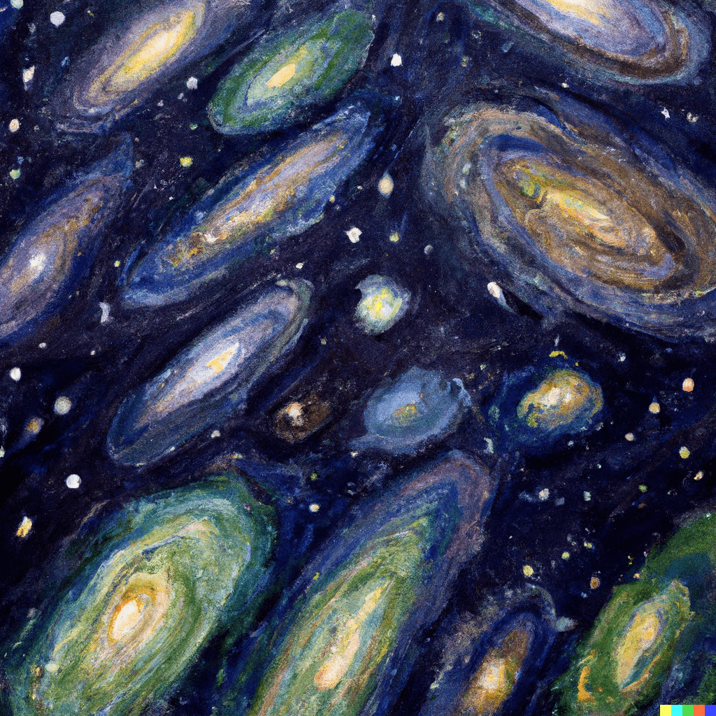
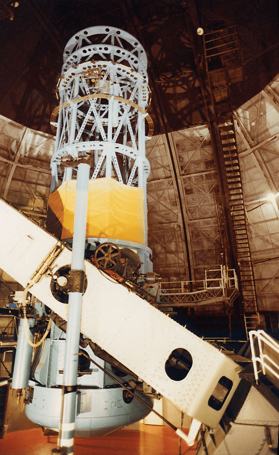
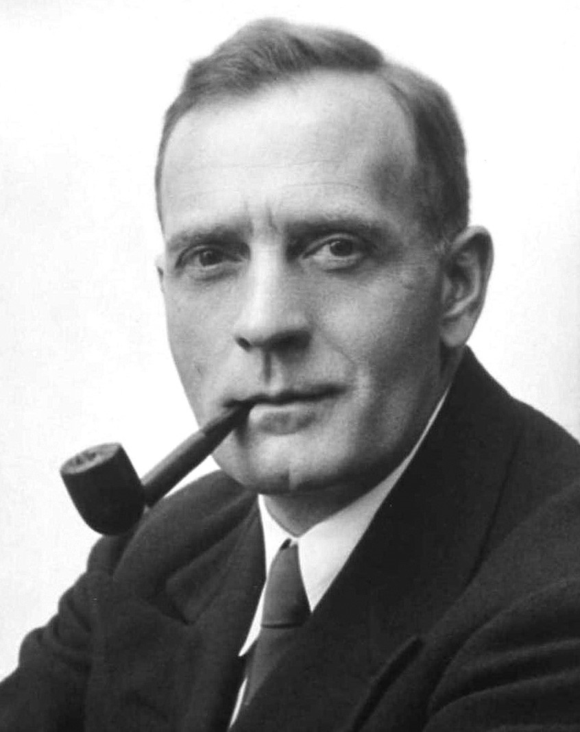
- 1924, Mount Wilson: Edwin Hubble shows the existence of
galaxies (previoulsy nebulae) using cepheids
Cataloguing galaxies
Cataloguing galaxies
- 1924, Mount Wilson: Edwin Hubble shows the existence of
galaxies (previoulsy nebulae) using cepheids - early imaging surveys carried out with photographic plates:
- 1949 - 1958: Palomar Observatory Sky Survey (POSS I)
- 1974 - 1999: UKST sky surveys, Siding Spring, Australia
- 1985 - 2000: POSS II
-
galaxy catalogs:
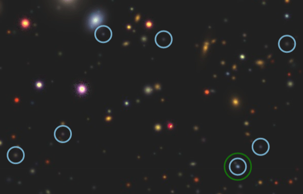
- 1961 - 1968: Zwicky Catalog of galaxies based on POSS I
- 1967: Lick catalog of 1 M galaxies
-
numerization:
- 1994: Digitized Sky Survey, scanning of POSS I/II and UKST: 102 CD-roms
- 1997 - 2001: 2MASS (Arizona, USA, and Chile) 3-band photometric survey
How to go 3D?
R.A.
Dec.
R.A.
Dec.
z
With spectroscopic surveys!
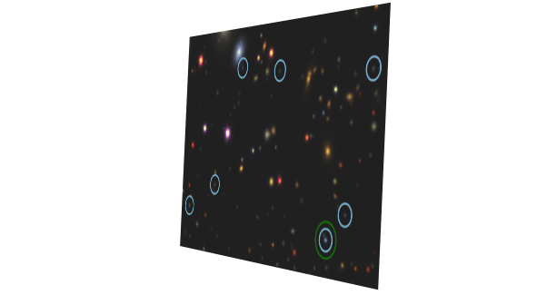
CfA redshift surveys
Mesurement of galaxy redshifts using a spectrograph.
- redshifts of galaxies from updated Zwicky catalogs
- 1977 - 1982: CfA I, 1100 redshifts, structures formed by galaxies
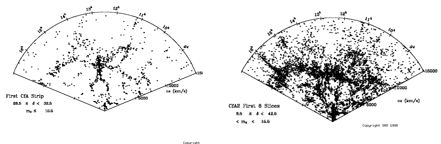
CfA redshift surveys
Mesurement of galaxy redshifts using a spectrograph.
- redshifts of galaxies from updated Zwicky catalogs
- 1977 - 1982: CfA I, 1100 redshifts, structures formed by galaxies
- 1985 - 1995: CfA II, 18 000 redshifts, Great Wall (Geller and Huchra 1989) at \(z \simeq 0.03\)
First cosmological constraints
- Vogeley et al. 1992 with CfA: inconsistency with CDM model at 99% (propose oCDM)
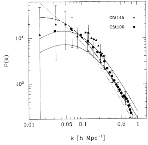
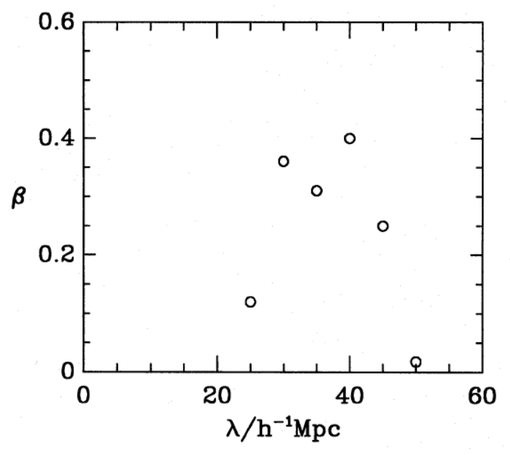
First cosmological constraints
- Vogeley et al. 1992 with CfA: inconsistency with CDM model at 99% (propose oCDM)
- Cole et al. 1994 with IRAS (infrared space telescope) data (15k redshifts): first measurement of anisotropy (\(\beta\) parameter) w.r.t. line-of-sight (due to redshift-space distortions)
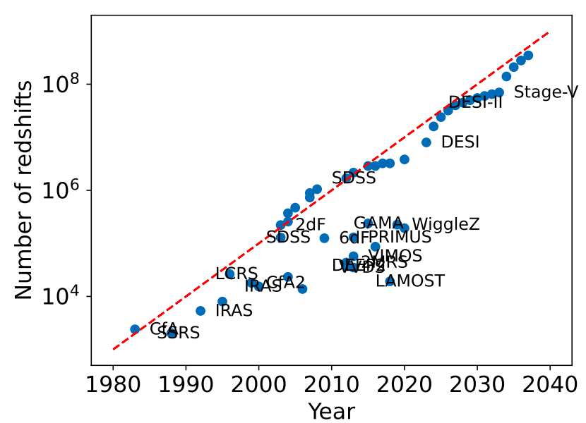
Large surveys
- made possible by multi-object spectroscopy
- high redshift (z > 0.5) surveys since 2005
Moore's law for spectroscopic surveys; Schlegel et al. 2022
Euclid
Outline
- History
- Observables and cosmological information
- Spectroscopic surveys and systematics
- Standard (RSD and BAO) analyses
- Current constraints
- On-going and future surveys
- Other clustering analyses
What do we measure?
We measure angular positions (right ascension (R.A.), declination
(Dec.)) and redshifts (\(z\)) of \(\mathcal{O}(10^6)\) galaxies.
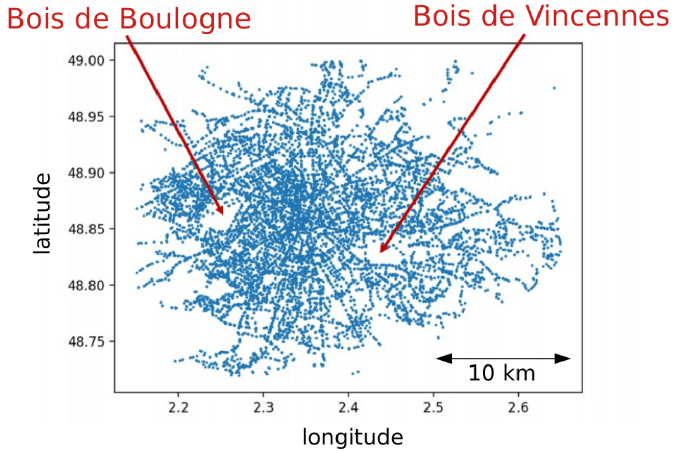
What to do with this data?
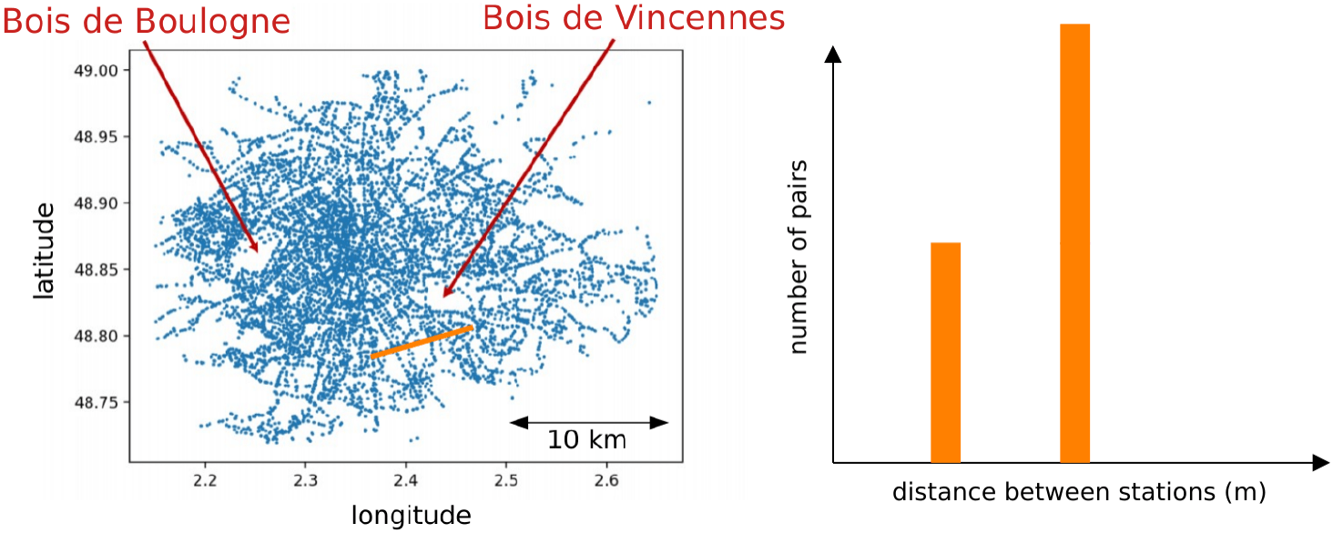
An example: Paris metro & bus stations
Credits: Etienne Burtin
Counting pairs
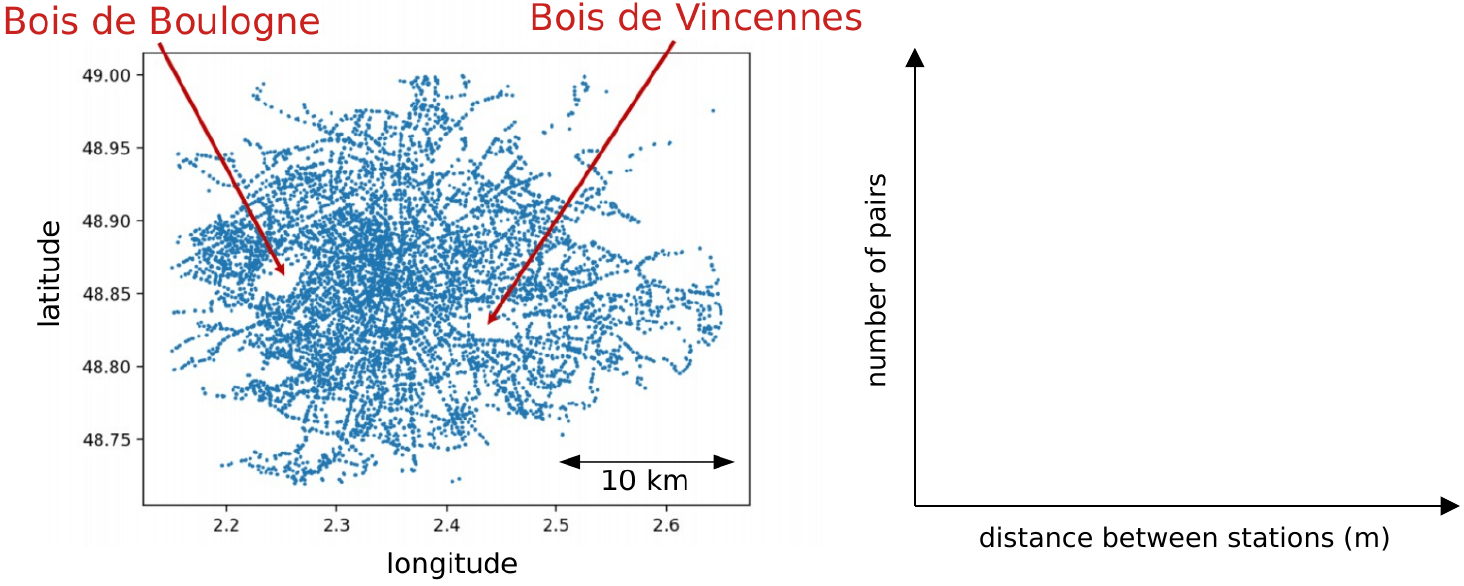
Counting pairs
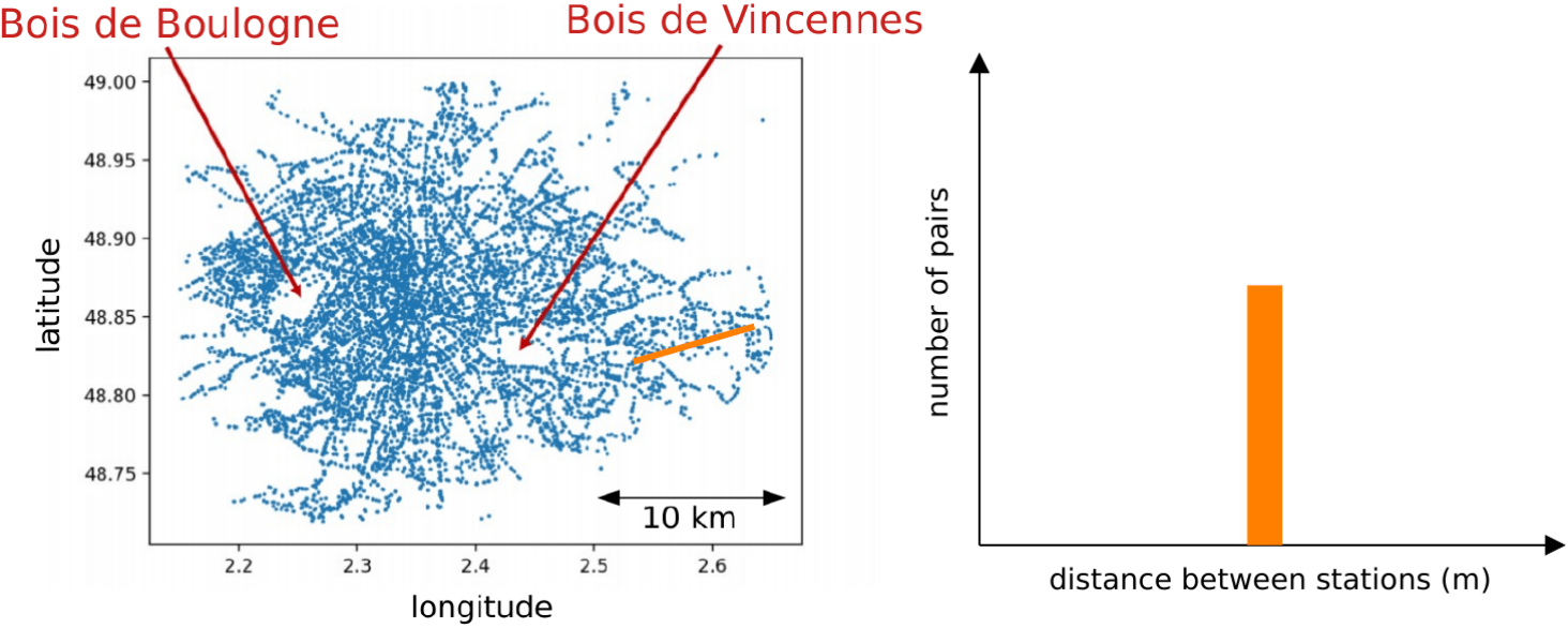
Counting pairs
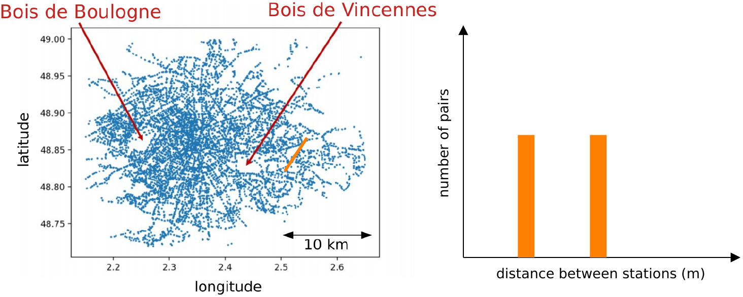
Counting pairs
Randoms
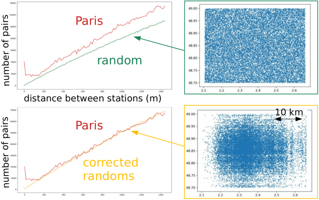
Randoms
Randoms
Credits: Etienne Burtin
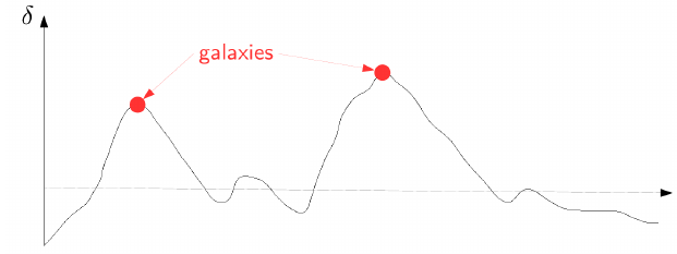
A bit of formalism
\(n_g(\mathbf{x}) = \bar{n}(\mathbf{x})\left[1 + \delta_g(\mathbf{x}) \right]\) \(\delta_g\) density contrast
Density of galaxies
Probability to find:
- one galaxy in \(dV_1\): \(dP_1 = \langle n_{g}(\mathbf{x}_1) dV_1 \rangle = \bar{n}(\mathbf{x}_1) dV_1\)
A bit of formalism
\(n_g(\mathbf{x}) = \bar{n}(\mathbf{x})\left[1 + \delta_g(\mathbf{x}) \right]\) \(\delta_g\) density contrast
Density of galaxies
Probability to find:
- one galaxy in \(dV_1\): \(dP_1 = \langle n_{g}(\mathbf{x}_1) dV_1 \rangle = \bar{n}(\mathbf{x}_1) dV_1\)
- two galaxies in \(dV_1\) and \(dV_2\):
\(\xi_{gg}(\mathbf{s}) = \left\langle \delta_g(\mathbf{x}_1) \delta_g(\mathbf{x}_1 + \mathbf{s}) \right\rangle\)
Covariance of the density contrast as a function of separation \(\mathbf{s}\)
Galaxy correlation function
Independent of position assuming spatial homogeneity.
Correlation function
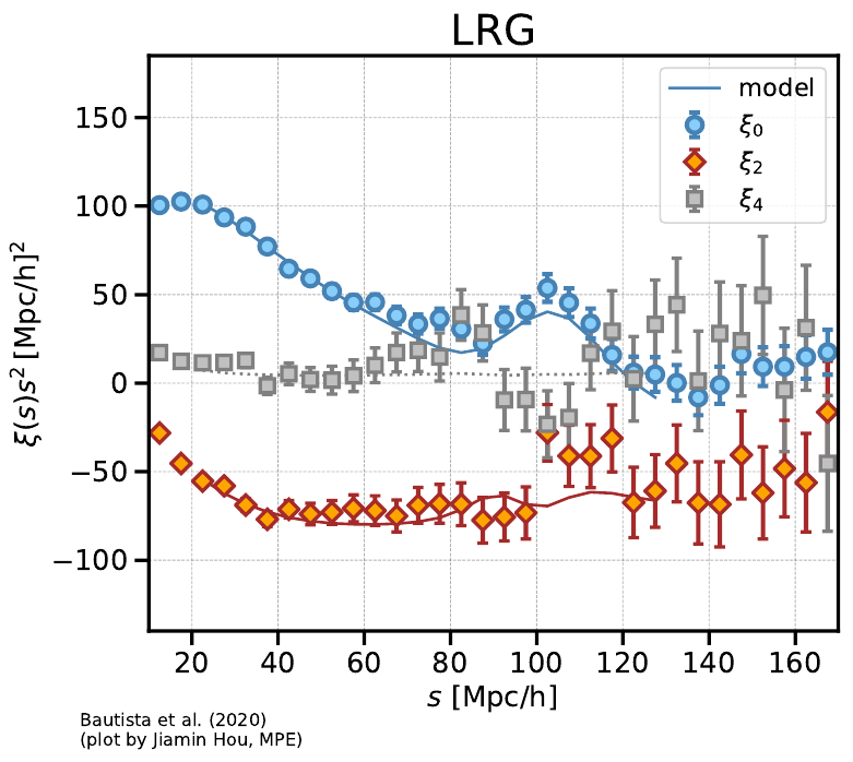
SDSS eBOSS DR16 LRG correlation function
Power spectrum
Fourier transform of the density contrast \(\delta_g(\mathbf{x})\)
\((2\pi)^3 \delta_D^{(3)}(\mathbf{k} + \mathbf{k}') P_{gg}(\mathbf{k}) = \langle \delta_g(\mathbf{k}) \delta_g(\mathbf{k}') \rangle\)
Galaxy power spectrum
- Dirac \(\delta_D^{(3)}(\mathbf{k} + \mathbf{k}')\) comes from homogeneity
- \(\xi_{gg}(\mathbf{s})\) and \(P_{gg}(\mathbf{k})\) are Fourier transform pairs:
Early time/large scales, \(\delta\) follows Gaussian statistics: fully described by 2-point function.
Power spectrum
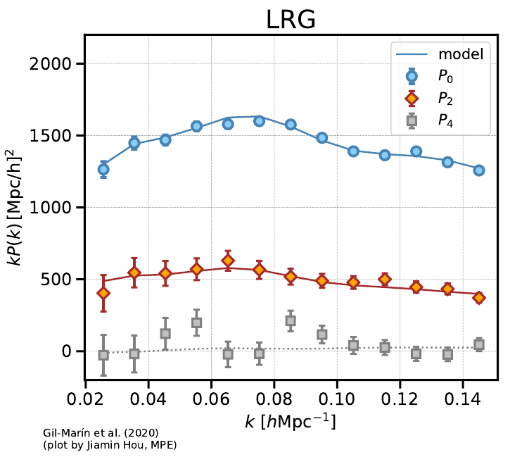
SDSS eBOSS DR16 LRG power spectrum
Galaxy - matter relation
How are \(\xi_{gg}(\mathbf{s})\) and \(P_{gg}(\mathbf{k})\) related to the (theory) matter power spectrum?
Galaxy bias
- galaxy formation in two steps (White and Rees 1978):
- dark matter forms halos (only gravity)
- gas cools down, baryons aggregate into galaxies
- galaxies trace the density field, in large overdensities → bias
Galaxy bias
- galaxy formation in two steps (White and Rees 1978):
- dark matter forms halos (only gravity)
- gas cools down, baryons aggregate into galaxies
- galaxies trace the density field, in large overdensities → bias
- perturbative expansion; at linear order \(\delta_g = b_1 \delta\), \(\delta\) matter field
- bottom-up approach (e.g. Seljak 2000):
- galaxies ⇔ DM halos with halo occupation distribution
- DM halos ⇔ DM field with halo bias (Sheth and Tormen 1999)
Features
What are the noticeable features in \(\xi_{gg}\) or \(P_{gg}\)?
Features
What are the noticeable features in \(\xi_{gg}\) or \(P_{gg}\)?
peak
oscillations
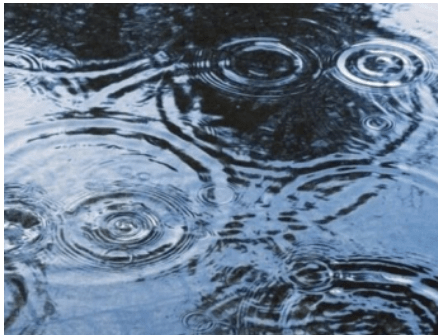
Baryon acoustic oscillations (BAO)
- before photon decoupling (CMB emission), acoustic waves propagated in a plasma of baryons and photons
Credits: CAASTRO, https://www.youtube.com/watch?v=jpXuYc-wzk4
Baryon acoustic oscillations (BAO)
- before photon decoupling (CMB emission), acoustic waves propagated in a plasma of baryons and photons
- baryon acoustic oscillations (BAO) imprinted in the CMB...
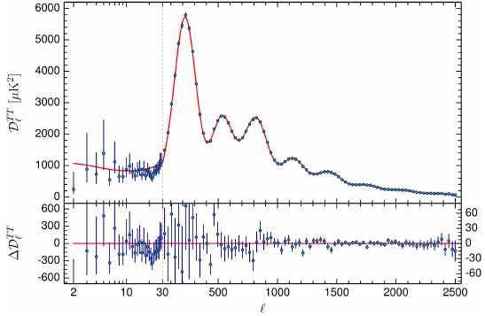
Credits: Esa & Planck
Baryon acoustic oscillations (BAO)
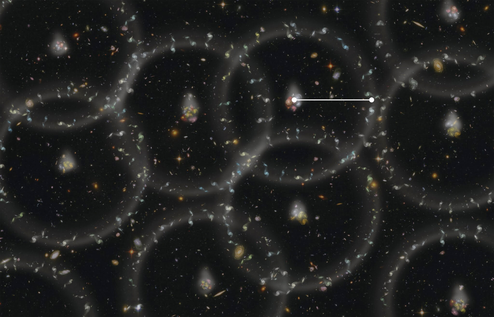
- ...and in the matter distribution at a fixed comoving scale: sound horizon at the drag epoch \(r_\mathrm{d}\)
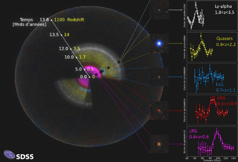
Baryon acoustic oscillations (BAO)
- ...and in the matter distribution at a fixed comoving scale: sound horizon at the drag epoch \(r_\mathrm{d}\)
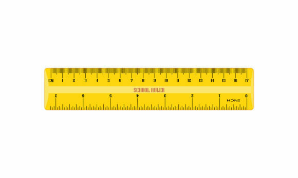
= standard ruler
Baryon acoustic oscillations (BAO)
In practice: catalog of angular positions and redshifts, so we constrain:
- angle on the sky (transverse to the line-of-sight): \(\theta_\mathrm{BAO} = D_\mathrm{M}(z) / r_\mathrm{d}\)
- \(\Delta z\) (along the line-of-sight): \( \Delta z_\mathrm{BAO} = r_\mathrm{d} / D_\mathrm{H}(z) = H(z) r_\mathrm{d} / c \)
transverse comoving distance
sound horizon \(r_d\)
Baryon acoustic oscillations (BAO)
In practice: catalog of angular positions and redshifts, so we constrain:
- angle on the sky (transverse to the line-of-sight): \(\theta_\mathrm{BAO} = D_\mathrm{M}(z) / r_\mathrm{d}\)
- \(\Delta z\) (along the line-of-sight): \( \Delta z_\mathrm{BAO} = r_\mathrm{d} / D_\mathrm{H}(z) = H(z) r_\mathrm{d} / c \)
Hubble distance
sound horizon \(r_d\)
Baryon acoustic oscillations (BAO)
In practice: catalog of angular positions and redshifts, so we constrain:
- angle on the sky (transverse to the line-of-sight): \(\theta_\mathrm{BAO} = \orange{D_\mathrm{M}(z)} / \green{r_\mathrm{d}}\)
- \(\Delta z\) (along the line-of-sight): \( \Delta z_\mathrm{BAO} = r_\mathrm{d} / D_\mathrm{H}(z) = \orange{H(z)} \green{r_\mathrm{d}} / c \)
- at multiple redshifts \(z\)
Probes the expansion history (\(\orange{D_\mathrm{M}, H}\)), hence the energy content (e.g. dark energy)
Absolute size at \(z = 0\): \(H_0 \green{r_d}\)
Features
What are the noticeable features in \(\xi_{gg}\) or \(P_{gg}\)?
non-zero quadrupole
Redshift space distortions (RSD)
observed redshifts (\(z_\mathrm{obs}\)) =
Hubble flow (\(z_\mathrm{cosmo}\))
+ peculiar velocities (\(u_z/(ac)\))
+ (relativistic terms)
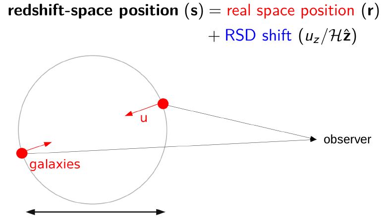
redshift-space positions (\(\mathbf{s}\)) =
real space position (\(\mathbf{r}\))
+ RSD shift (\(u_z/\mathcal{H}\mathbf{\hat{z}}\))
Redshift space distortions (RSD)
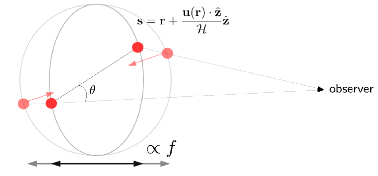
dependence in \(\mu = \cos \theta\) cosine angle to the line-of-sight
Legendre expansion in multipoles (usually truncated at \(\ell = 4\)):
Redshift space distortions (RSD)
galaxy positions in redshift space: \(\mathbf{s} = \mathbf{r} - v_z \hat{z}\) with \(v_z = -\frac{\mathbf{u} \cdot \hat{z}}{\mathcal{H}}\)
mass conservation:
\([1 + \delta_s(\mathbf{s})] d^3s = [1 + \delta_r(\mathbf{r})] d^3r \implies \delta_s(\mathbf{s}) = \left[ 1 + \delta_r(\mathbf{r}) \right] \left| \frac{d^3 s}{d^3 r} \right|^{-1} - 1 \)
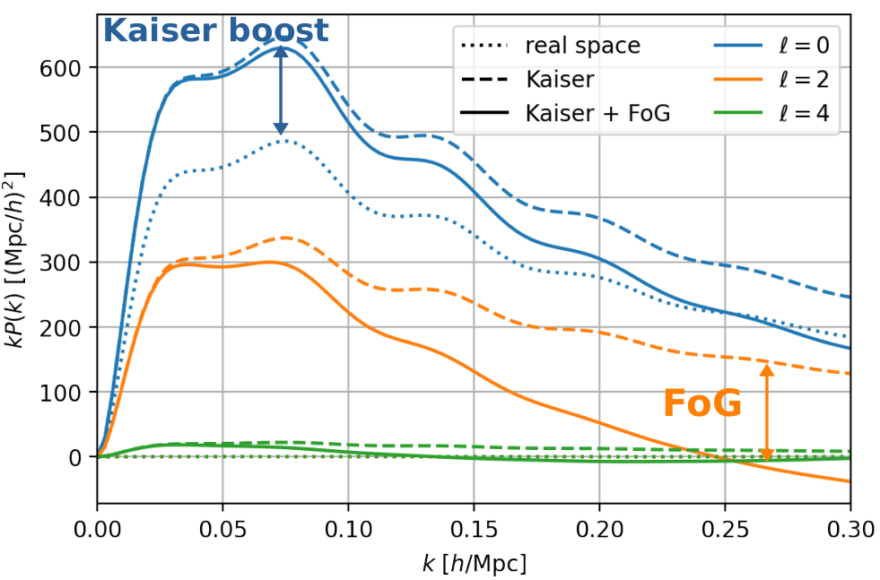
power spectrum in redshift space:
Kaiser: \(\delta_r + \partial_z v_z \rightarrow (b_1 + f \mu^2)\delta\) in linear theory, enhancement on large scales
Finger-of-God: \(e^{-ik_\mu \Delta v_z}\) damping on scales \(\lesssim 3\, \mathrm{Mpc}\)
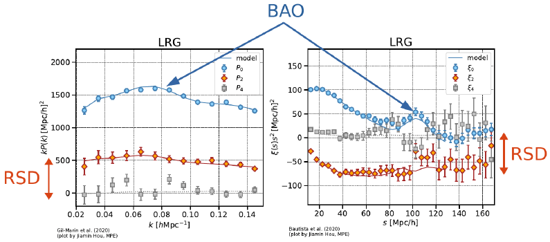
Measurement of \(f\sigma_8\)
\(P_s(k, \mu) = (b_1 + f \mu^2)^2 P_{\delta\delta}(k) = b_1^2 (1 + \beta \mu^2)^2 P_{\delta\delta}(k)\)
Kaiser model
with \(\beta = f / b_1\). Equivalently:
(for historical reasons) at a pivot point of \(8\;\mathrm{Mpc}/h\)
\(= f \sigma_8\) with \(f = \frac{d \ln D}{d \ln a} \simeq \Omega_m^{0.55}\) within ΛCDM
probe matter density \(\Omega_m\) / test of general relativity
Typically bias is marginalised over:
effectively measure the (amplitude of) the velocity divergence power spectrum \(P_{\theta\theta}(k)\)
Summary
Measurement of the anisotropic correlation function or power spectrum of galaxies. Sensitive to:
- RSD: \(f\sigma_8\) ⇒ energy content, test of general relativity
- BAO: \(D_M / r_\mathrm{d} , D_H /r_\mathrm{d}\) ⇒ energy content
- more generally: primordial power spectrum (inflation, matter-radiation equality), neutrinos, etc.
Standard clustering analyses
Estimators
How to compute \(\xi_{gg}\) or \(P_{gg}\) from a galaxy catalog?
Correlation function estimators
Let \(XY(\mathbf{s})\) be the (normalized, weighted) number of pairs of objects from catalogs \(X, Y\) as a function of separation \(\mathrm{s}\)
Correlation function estimators
Let \(XY(\mathbf{s})\) be the (normalized, weighted) number of pairs of objects from catalogs \(X, Y\) as a function of separation \(\mathrm{s}\)
\(\hat{\xi}_g(\mathbf{s}) = \frac{DD(\mathbf{s})}{RR(\mathbf{s})} − 1\) minimally biased but large variance
Natural estimator
\(\hat{\xi}_g(\mathbf{s}) = \frac{DD(\mathbf{s})}{DR(\mathbf{s})} − 1\) biased and not minimal variance
Davis and Peebles 1983 estimator
\(\hat{\xi}_g(\mathbf{s}) = \frac{DD(\mathbf{s}) RR(\mathbf{s})}{DR(\mathbf{s})^2} − 1\) minimal variance but biased
Hamilton 1993 estimator
Correlation function estimators
\(\hat{\xi}_g(\mathbf{s}) = \frac{DD(\mathbf{s})}{RR(\mathbf{s})} − 1\) minimally biased but large variance
Natural estimator
\(\hat{\xi}_g(\mathbf{s}) = \frac{DD(\mathbf{s})}{DR(\mathbf{s})} − 1\) biased and not minimal variance
Davis and Peebles 1983 estimator
\(\hat{\xi}_g(\mathbf{s}) = \frac{DD(\mathbf{s}) RR(\mathbf{s})}{DR(\mathbf{s})^2} − 1\) minimal variance but biased
Hamilton 1993 estimator
\(\hat{\xi}_g(\mathbf{s}) = \frac{DD(\mathbf{s}) - 2DR(\mathbf{s}) + RR(\mathbf{s})}{RR(\mathbf{s})}\) minimally biased, minimal variance
Landy-Szalay 1993 estimator
Let \(XY(\mathbf{s})\) be the (normalized, weighted) number of pairs of objects from catalogs \(X, Y\) as a function of separation \(\mathrm{s}\)
Power spectrum estimator
\(F(\mathbf{x}) = n_g(\mathbf{x}) − \bar{n}(\mathbf{x})\)
Density fluctuations
Yamamoto 2006 estimator
with:
Power spectrum estimator
\(F(\mathbf{x}) = n_g(\mathbf{x}) − \bar{n}(\mathbf{x})\)
Density fluctuations
Yamamoto 2006 estimator
with:
- \(F_\ell(\mathbf{k})\) ⇒ simple Fourier transforms
- \(F\) (galaxies, randoms) painted on a mesh for FFT
- aliasing effects
- shotnoise \(P_\ell^\mathrm{noise}(k_\mu) \simeq \delta_{\ell 0}^{K} \bar{n}^{-1}\) : subtracted as galaxies assumed to be a ∼ Poisson sampling of the dark matter field
Window function effect
Survey has finite size: window function effect
- correlation function: already corrected for by the \(RR(s, \mu)\) term in the denominator
- power spectrum: to be deconvolved, or included in power spectrum model: matrix multiplication (e.g. Beutler and McDonald 2021) \(W_{\alpha\beta} = d\langle \hat{P}_\alpha \rangle / d P_\beta\)
- other effects: wide-angle, integral constraints (Beutler et al. 2019; de Mattia and Ruhlmann-Kleider 2019)
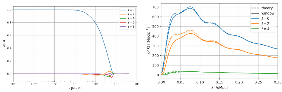
For a \(6\; \mathrm{Gpc}/h\) box
Measurement covariance
Power spectrum covariance is, using Wick’s theorem (Gaussian field):
with \(\mu = \mathbf{\hat{k}} \cdot \mathbf{\hat{x}}\)
minimizing variance: FKP (Feldman et al. 1994) weights
\(w_\mathrm{FKP} = 1/ [1 + \bar{n}(z)P_0)]\) applied to galaxies (and randoms)
Measurement covariance
Power spectrum covariance is, using Wick’s theorem (Gaussian field):
- covariance matrix typically estimated from mocks: fast simulations of the galaxy density field, including survey selection function
- noise in the covariance matrix: noise in the cosmological measurement. Artificially enlarge error bars (Hartlap et al. 2007; Percival et al. 2014; Percival et al. 2022)
- accurate analytic estimations are developed
with \(\mu = \mathbf{\hat{k}} \cdot \mathbf{\hat{x}}\)
minimizing variance: FKP (Feldman et al. 1994) weights
\(w_\mathrm{FKP} = 1/ [1 + \bar{n}(z)P_0)]\) applied to galaxies (and randoms)
Measurement covariance
In the uniform \(\bar{n}\) limit:
- larger survey volume: \(\mathrm{error} \propto 1/\textcolor{blue}{V_s}\)
- higher density: \(\mathrm{error} \propto 1/\textcolor{red}{\bar{n}}\) when in the shot-noise dominated regime \(\bar{n} \ll 1/P_0\)
Two leverages to minimize variance (= higher measurement precision):
Credit: DESI
Outline
- History
- Observables and cosmological information
- Spectroscopic surveys and systematics
- Standard (RSD and BAO) analyses
- Current constraints
- On-going and future surveys
- Other clustering analyses
Spectroscopic galaxy surveys


imaging surveys (2014 - 2019) + WISE (IR)
target selection
spectroscopic observations
spectra and redshift measurements
- two steps: photometry and spectroscopy ⇒ selection effects
- catalog of angular positions \(\mathrm{R.A.}, \mathrm{Dec.}\) and redshifts \(z\)
Survey selection function
specify the survey selection function \(\bar{n}\) ⇒ account for systematic effects due to photometry/spectroscopy
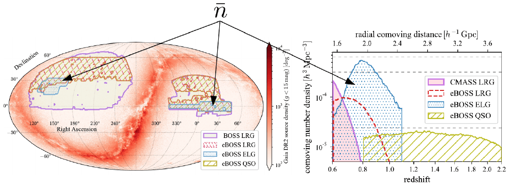
Taken from Zhao et al. (2020)
Expected density without clustering = angular & radial footprint
Survey selection function
Photometry
- photometric surveys: images of the sky, taken with different filters
- mainly characterized by their depth (magnitude corresponding to given probability of source detection), seeing (size of PSF)
- pipeline for source detection and source fitting (flux, shape, etc.)
- Legacy Surveys: https://www.legacysurvey.org/viewer
Taken from Zhao et al. (2020)
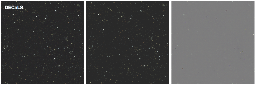
From left to right: data, model, residual. From Dey et al. (2019) (DECaLS DR8).
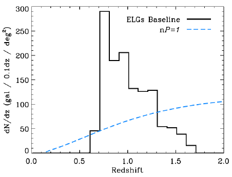
Target selection
- to obtain objects of certain class (luminous red galaxies, emission line galaxies, quasars...) in a redshift range
- typically with cuts in colour and magnitude
Taken from Zhao et al. (2020)
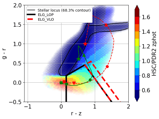
c) high-z
b) star / low-z rejection
d) [OII]
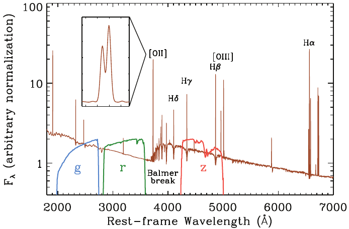
Left: taken from Raichoor et al. (2022). Right: taken from DESI Collaboration et al. (2016).
Photometric systematics
- veto masks in selection function n̄ for bright objects, (variable) stars, bad pixels...
-
target density varies with observational conditions: depth,
seeing, galaxy extinction, star density... to be modelled
Taken from Zhao et al. (2020)
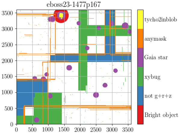
Left: masks on a legacypipe \(0.25^\circ × 0.25^\circ\) brick.
Taken from Raichoor et al. (2020).
Fiber collisions
- Fiber-fed spectrographs: fibers cannot be too close (e.g. 62'′ for SDSS) / "fixed density of fibers"
- SDSS-I < IV: hand-plugged fibers
- WiggleZ: fibers positioned by a robot
- SDSS V, DESI: robotic positioner for each fiber
Taken from Zhao et al. (2020)
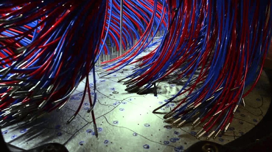
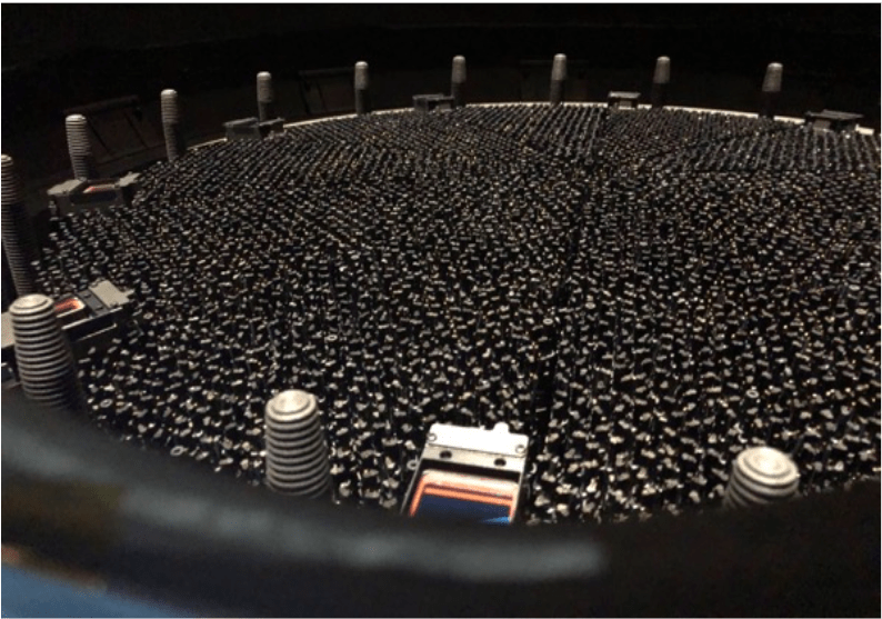
Credit: SDSS
Credit: DESI
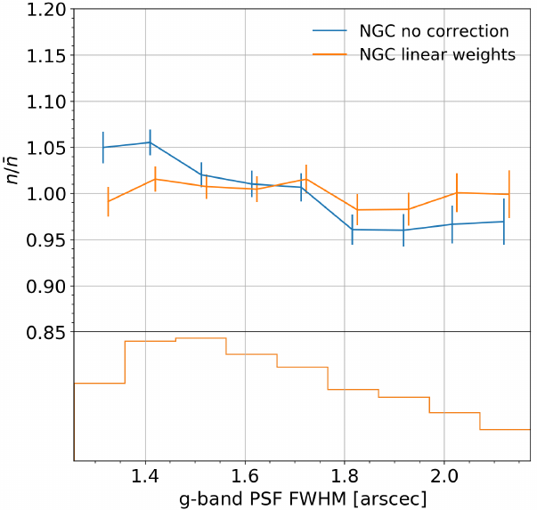
Fiber collisions
- density-dependent effect: correlates with clustering
Taken from Zhao et al. (2020)
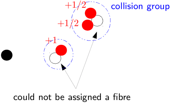
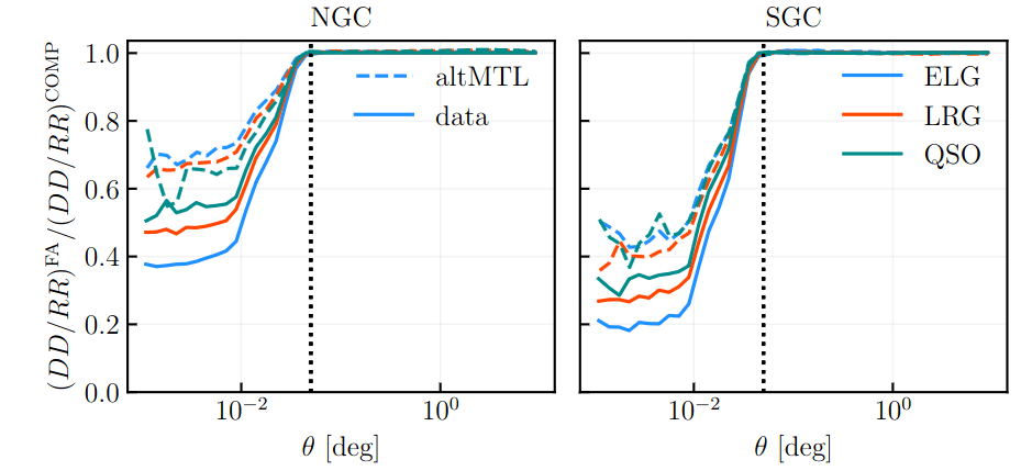
individual galaxy weights not sufficient:
- pairwise inverse probability weights (PIP) (e.g. Bianchi and Percival 2017): rerun fiber assignment many times with different random seeds
- \(\theta\)-cut: remove all small scale angular pairs (e.g. Pinon et al. 2024)
\(0.05^\circ \simeq\) positioner patrol diameter
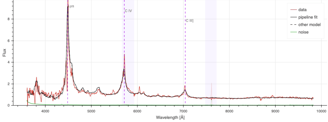
Spectroscopic measurements
Taken from Zhao et al. (2020)
- grims disperse light onto the focal plane
- reduction of 2D traces into 1D
- spectrum fit with a basis of archetypes / PCA templates
- criterion to select reliable redshifts
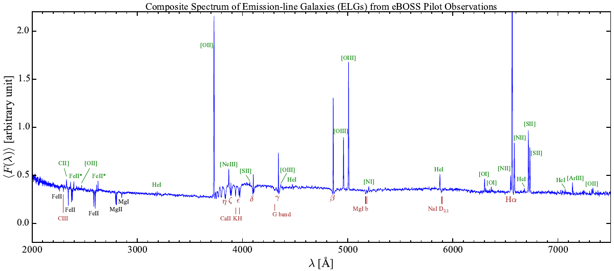
Taken from Zhu et al. 2015
Redshift failures
Taken from Zhao et al. (2020)
- redshift efficiency involves the response of the telescope,
spectrograph and redshift determination pipeline - may vary with spectroscopic observing conditions / instrument
- corrected by a weight
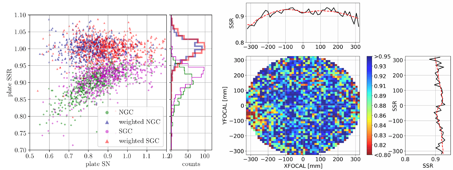
Taken from Raichoor et al. 2020
Summary
Taken from Zhao et al. (2020)
\(\bar{n}\) varies due to photometry and spectroscopy:
- angular photometric systematics
- fibre collisions
- redshift failures
Understanding \(\bar{n}\) is key to reliable clustering measurements.
Effects of systematics tested on fast simulations: mocks.
Survey selection function
Taken from Zhao et al. (2020)
Outline
- History
- Observables and cosmological information
- Spectroscopic surveys and systematics
- Standard (RSD and BAO) analyses
- Current constraints
- On-going and future surveys
- Other clustering analyses
Taken from Zhao et al. (2020)
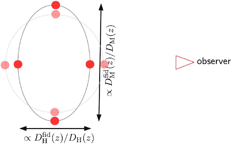
Alcock-Paczynski effect
angular positions \((\mathrm{R.A.}, \mathrm{Dec.})\) and redshifts \(z\) of galaxies converted into Cartesian coordinates assuming a fiducial cosmology (\(\mathrm{fid}\))
In the model, wavevectors in the true cosmology ⇒ fiducial cosmology, multiply by:
Taken from Zhao et al. (2020)
BAO model
- only measuring position of the BAO peak: robust
- split fiducial power spectrum \(P(k)\) into no-wiggle \(P_\mathrm{nw}(k)\) and wiggles \(P_\mathrm{w}(k) = P(k) - P_\mathrm{nw}(k)\)
- marginalize over the shape: broadband parameters (polynomials)
- adjust position of wiggles \(P_\mathrm{w}(k^\prime = k / \alpha)\)

"no-wiggle Kaiser"
Taken from Zhao et al. (2020)
BAO model
- only measuring position of the BAO peak: robust
- split fiducial power spectrum \(P(k)\) into no-wiggle \(P_\mathrm{nw}(k)\) and wiggles \(P_\mathrm{w}(k) = P(k) - P_\mathrm{nw}(k)\)
- marginalize over the shape: broadband parameters (polynomials)
- adjust position of wiggles \(P_\mathrm{w}(k^\prime = k / \alpha)\)
- correlation function: Hankel transform of \(P_{gg}(k)\)
Taken from Zhao et al. (2020)
BAO model
If enough S/N: also fit quadrupole to measure anisotropic BAO \(\alpha_\parallel / \alpha_\perp = D_\mathrm{H} / D_\mathrm{M}\)


\(P_{gg}\)
\(\xi_{gg}\)
\(P_{gg}\)
monopole
quadrupole
monopole
quadrupole
Non-linear structure growth and peculiar velocities blur and shrink (slightly) the ruler

Eisenstein et al. 2008, Padmanabhan et al. 2012
BAO reconstruction
Estimates Zeldovich displacements from observed field and moves galaxies back: refurbishes the ruler (improves precision and accuracy)
reconstruction
BAO reconstruction
Taken from Zhao et al. (2020)
RSD models
Unbiased measurement of amplitude \(f\sigma_8\) ⇒ accurate model for the full shape power spectrum.
Various approaches (% accuracy at \(z = 1\)):
- WiggleZ (Blake, 2010): Halofit \(P_m(k)\) + Kaiser + FoG
- in BOSS/eBOSS (< 2020): perturbation theory models:
- power spectrum: standard/regularized PT (RPT, RegPT Taruya et al. 2012), RSD (Taruya et al. 2010), bias expansion (McDonald and Roy 2009) (\(k < 0.2 \; h/\mathrm{Mpc}\))
- correlation function: Gaussian streaming model (Reid and White 2011) (\(s > 30 \; \mathrm{Mpc}/h\))
Taken from Zhao et al. (2020)
RSD models
Unbiased measurement of amplitude \(f\sigma_8\) ⇒ accurate model for the full shape power spectrum.
Various approaches (% accuracy at \(z = 1\)):
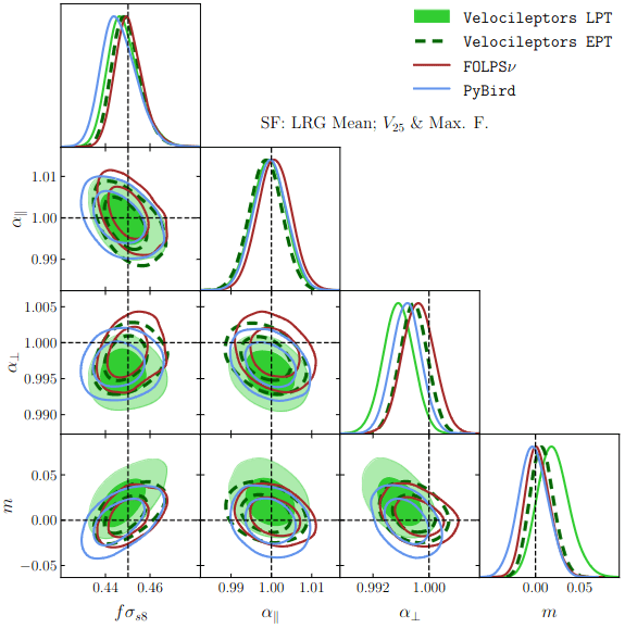
- for DESI, Euclid, effective field theory: small scale sourced counterterm to regularize loop integrals (pybird, CLASS-PT, velocileptors, folps...) (\(k < 0.25 \; h/\mathrm{Mpc}\))
counterterms
stochastic terms
SPT
Taken from Zhao et al. (2020)
RSD models
Unbiased measurement of amplitude \(f\sigma_8\) ⇒ accurate model for the full shape power spectrum.
Various approaches (% accuracy at \(z = 1\)):
- for DESI, Euclid, effective field theory: small scale sourced counterterm to regularize loop integrals (pybird, CLASS-PT, velocileptors, folps...) (\(k < 0.25 \; h/\mathrm{Mpc}\))
- also hybrid PT/HOD models, e.g. Hand et al. 2017 (\(k < 0.4 \; h/\mathrm{Mpc}\))
- simulation-based models, e.g. SimBig Lemos et al. 2023
counterterms
stochastic terms
SPT
Taken from Zhao et al. (2020)
Testing models: N-body mock challenge
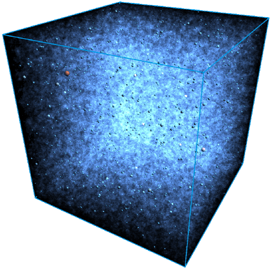
Snapshot of the OuterRim simulation at \(z = 0\). Taken from Heitmann et al. (2019).
solve numerically the Vlasov-Poisson equations for the dark matter fluid by sampling the phase-space with particles
N-body simulations
- \(10,240^3\) DM particles, \(1.85 \times 10^9 M_\odot/h\)
- particles clustered in halos, found with a Friend-of-Friend algorithm
OuterRim simulation
Taken from Zhao et al. (2020)
Halo occupation distribution
specify the probability to find N galaxies in a halo of mass M
Halo occupation distribution
- usually split between central and satellite galaxies
- typically tuned to reproduce semi-analytic models of galaxy formation (SAM) and observational data
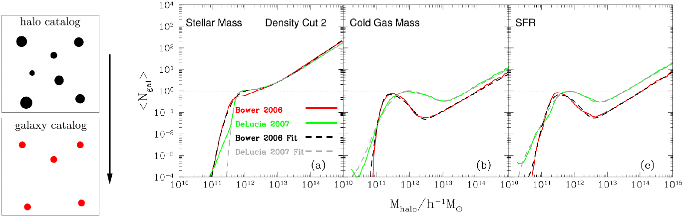
Right: HOD measured on the outputs of two semi-analytical models (GALFORM and LGALAXIES) run on the Millennium simulation. Taken from Contreras et al. (2013).
other approach: sub-halo abundance matching (SHAM)
Taken from Zhao et al. (2020)
Mock challenge
Test the theoretical model accuracy against simulations (mocks)
Mock challenge
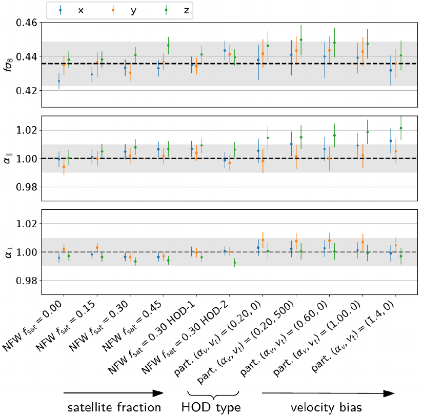
- vary HOD shape, satellite fraction, positions and velocities, probability laws...
- e.g.: ELG in halo outskirts,
infalling velocities
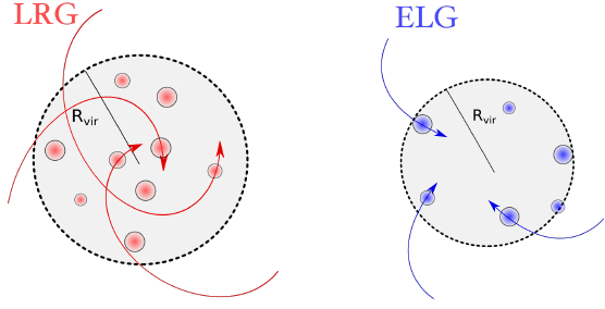
Taken from Orsi and Angulo (2018)
Summary
Taken from Zhao et al. (2020)
- BAO models: marginalize over the shape of the power spectrum ("broadband")
- RSD models: full shape of the power spectrum up to midly non-linear scales
- tested with N-body mock challenge
Theory models
Taken from Zhao et al. (2020)
Outline
- History
- Observables and cosmological information
- Spectroscopic surveys and systematics
- Standard (RSD and BAO) analyses
- Current constraints
- On-going and future surveys
- Other clustering analyses
Taken from Zhao et al. (2020)
BAO
6dFGRS
SDSS (MGS)
SDSS (BOSS/eBOSS)
WiggleZ


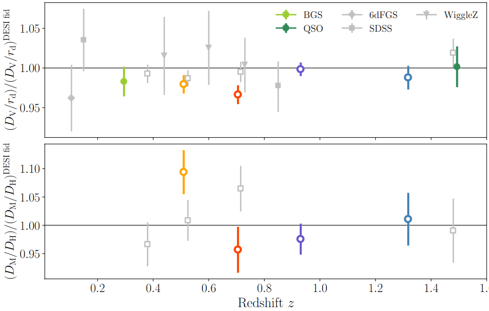
DESI Y1 BAO measurements
BAO (DESI)
DESI Y1 BAO measurements


BAO (DESI)
DESI Y1 BAO measurements


BAO (DESI)
DESI Y1 BAO measurements


BAO (DESI)
DESI Y1 BAO measurements

Consistent with each other,
and complementary
BAO (DESI)
BAO constraints (DESI, SDSS) consistent with CMB (primary and lensing Planck Collaboration, 2018, ACT Collaboration, 2023, Carron, Mirmelstein, Lewis, 2022)

BAO (DESI)
BAO (DESI)
- BAO constrains \( r_\mathrm{d}(\blue{\Omega_\mathrm{m}} h^{2}, \orange{\Omega_\mathrm{b} h^{2}}) h \)
- \( \blue{\Omega_\mathrm{m}} \) constrained by BAO at different \(z\)
- \(\orange{\Omega_\mathrm{b}h^2}\) can be constrained by light element abundance from Big Bang Nucleosynthesis (BBN): Schöneberg et al., 2024
\(\implies\) constraints on \(h\) i.e. \(H_0 = 100 h \; \mathrm{km} / \mathrm{s} / \mathrm{Mpc}\)

- SDSS / DESI consistency
- In agreement with CMB
- In \(3.7 \sigma\) tension with SH0ES
BAO (DESI)

BAO + CMB measurements favor a flat Universe
BAO (DESI)
Dark Energy fluid, pressure \(p\), density \(\rho\), Equation of State parameter \(w = p / \rho\)
BAO (DESI)
Dark Energy fluid, pressure \(p\), density \(\rho\), Equation of State parameter \(w = p / \rho\)
Assuming a constant EoS, DESI BAO fully compatible with a cosmological constant...

Constant EoS parameter \(w\)
BAO (DESI)
Dark Energy fluid, pressure \(p\), density \(\rho\), Equation of State parameter \(w = p / \rho\)

Varying EoS
BAO (DESI)
Internal CMB degeneracies limiting precision on the sum of neutrino masses
Broken by BAO, especially through \(H_{0}\)
Low preferred value of \(H_{0}\) yields
\(\sum m_\nu < 0.072 \, \mathrm{eV} \; (95\%, \color{green}{\text{DESI + CMB})}\)

Limit relaxed for extensions to \(\Lambda\mathrm{CDM}\)
\(\sum m_\nu < 0.195 \, \mathrm{eV}\) for \(w_0w_a\mathrm{CDM}\)
Taken from Zhao et al. (2020)
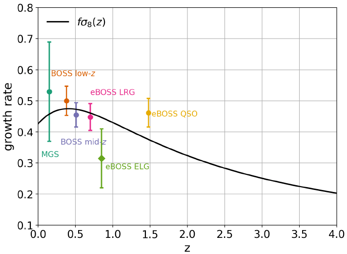
RSD (SDSS)
DESI RSD results are not yet published! Come back next year ;)
In the meantime, let's use SDSS!
Taken from Zhao et al. (2020)
RSD (SDSS)
- RSD constrain structure growth, competitive with weak lensing
Taken from Zhao et al. (2020)
RSD (SDSS)
- RSD constrain structure growth, competitive with weak lensing
With DESI Y1...
Taken from Zhao et al. (2020)
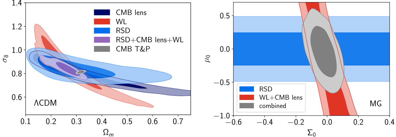
RSD (SDSS)
- RSD constrain structure growth, competitive with weak lensing
- RSD constrain deviations to GR e.g.
- complementary to weak lensing and CMB lensing
Taken from Zhao et al. (2020)
Outline
- History
- Observables and cosmological information
- Spectroscopic surveys and systematics
- Standard (RSD and BAO) analyses
- Current constraints
- On-going and future surveys
- Other clustering analyses
Taken from Zhao et al. (2020)
Euclid (spectro)
\(15 000 \; \mathrm{deg}²\), 50M H\(\alpha\) emitters between \(0.9 < z < 1.8\)
slitless spectroscopy with NISP, R = \(\lambda / \Delta \lambda\) = 380
just launched!
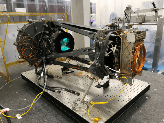
NISP instrument. Euclid consortium
Taken from Zhao et al. (2020)
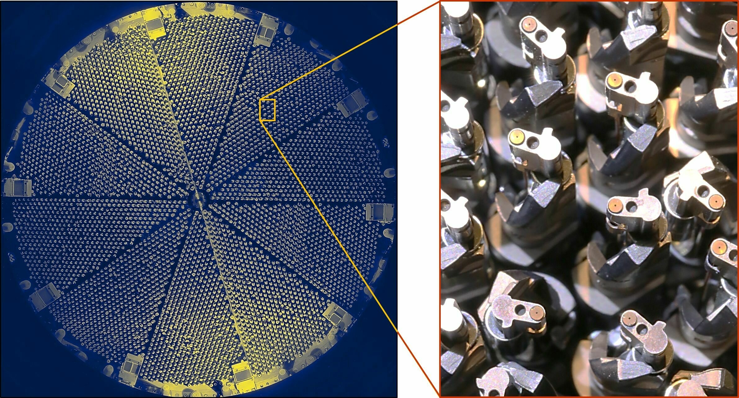
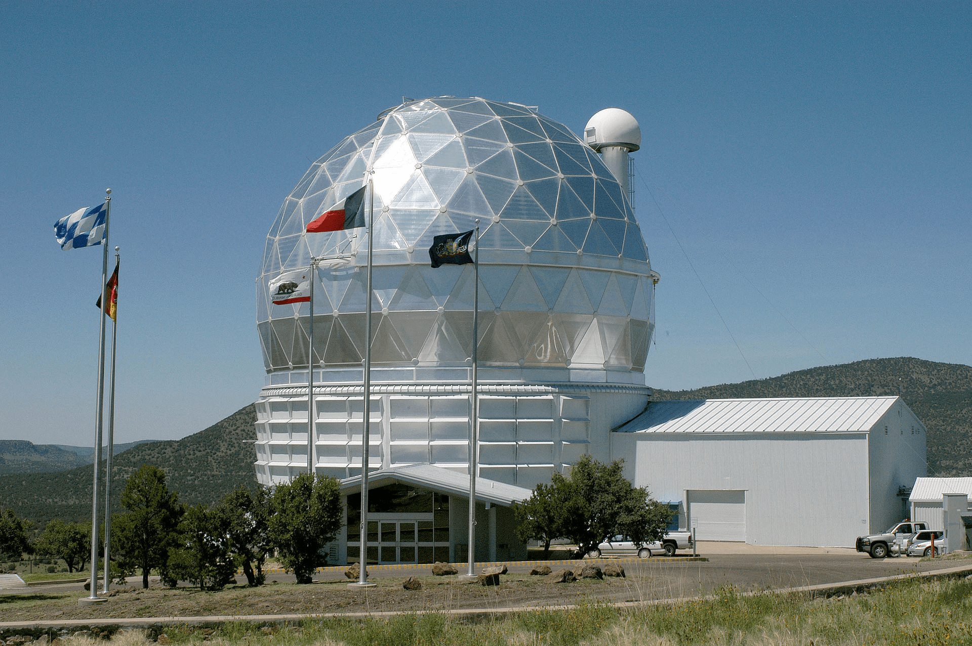
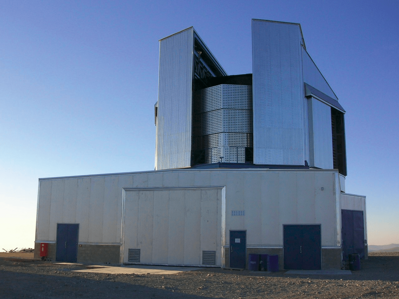
DESI
Mayall Telescope at Kitt Peak, AZ
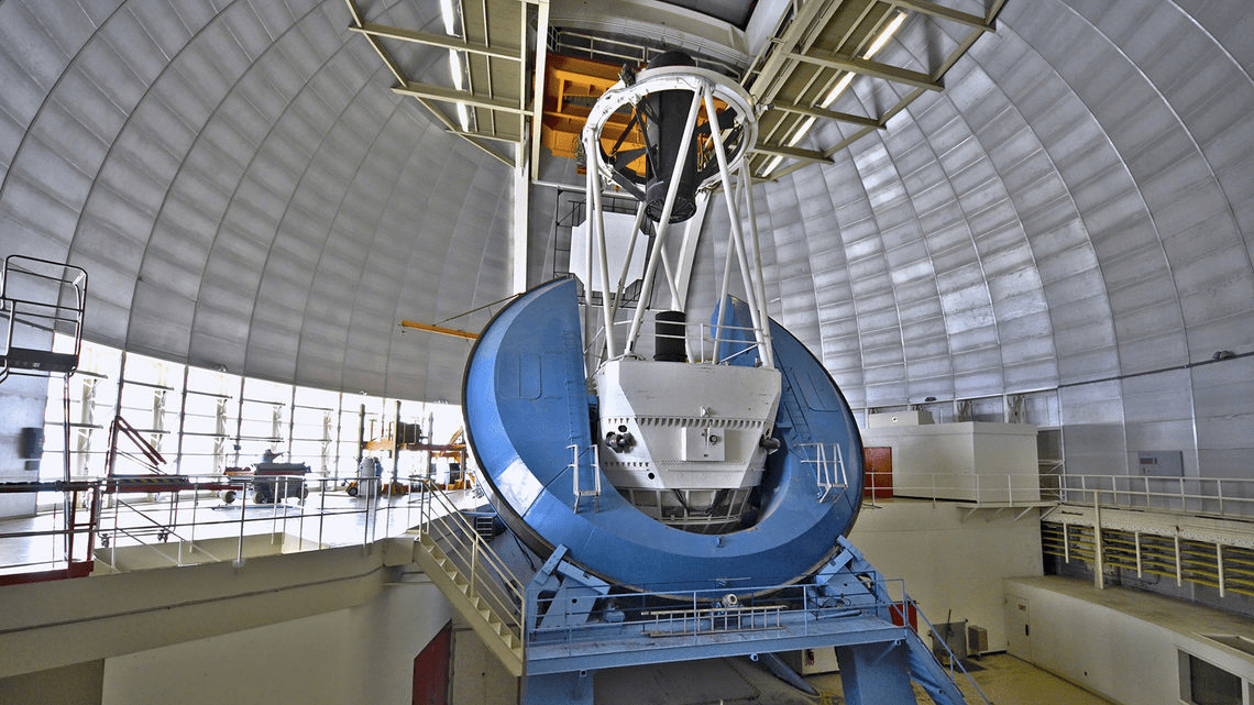
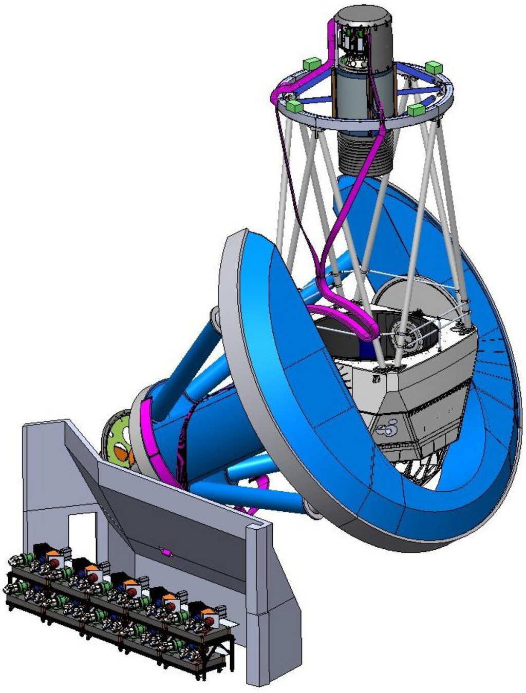
focal plane 5000 fibers
wide-field corrector
6 lenses, FoV \(\sim 8~\mathrm{deg}^{2}\)
4 m mirror
fiber view camera
ten 3-channel spectrographs
49 m, 10-cable fiber run
Taken from Zhao et al. (2020)
DESI
Credit: NSF
Taken from Zhao et al. (2020)
DESI focal plane

Taken from Zhao et al. (2020)
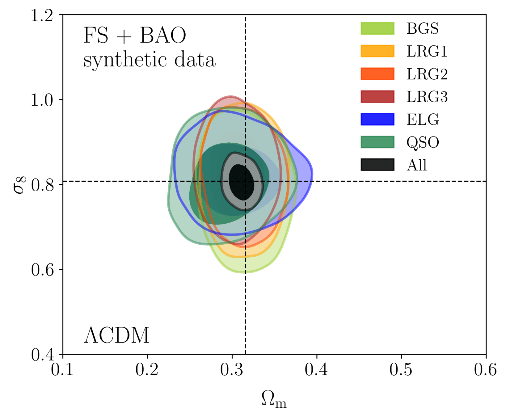
DESI Y5 galaxy samples
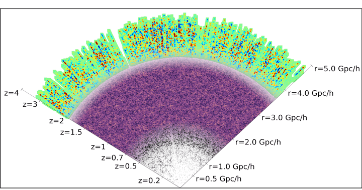
Bright Galaxies: 14M
0 < z < 0.4
LRG: 8M
0.4 < z < 0.8
ELG: 16M
0.6 < z < 1.6
QSO: 3M
Lya \(1.8 < z\)
Tracers \(0.8 < z < 2.1\)
\(z = 0.4\)
\(z = 0.8\)
\(z = 0\)
\(z = 1.6\)
\(z = 2.0\)
\(z = 3.0\)
Y5 \(\sim 40\)M galaxy redshifts!
Taken from Zhao et al. (2020)
Other redshift surveys
- HETDEX (2017-2023): 1M (Lyman-\(\alpha\) emitting) galaxies, untargeted survey (R ∼ 800)
- 4MOST (2024-2029): 25M spectra \(15,000\;\mathrm{deg}^2\)
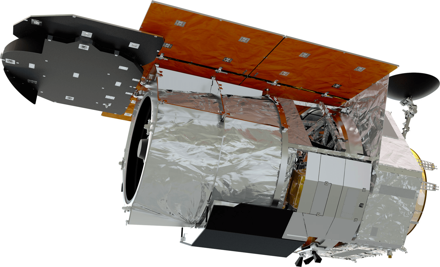
- Nancy-Grace-Roman / WFIRST (2025-2030): 20M H\(\alpha\) emitters (R = 70 − 140 and R = 450 − 850), slitless spectroscopy
Taken from Zhao et al. (2020)
Other clustering analyses
- small scales: HOD + cosmology fitting, e.g. Chapman et al. 2021
- large scales: primordial non-Gaussianity \(f_\mathrm{NL}\), scale-dependent \(\propto 1/k^2\) bias, e.g. Mueller et al. 2021
- higher order correlation functions (3-pt, 4-pt...): e.g. Slepian et al. 2017
- alternative clustering statistics: e.g. marked correlation function, density-split correlation function, e.g. Paillas et al. 2023
- field-level inference of the galaxy: density Lavaux et al. 2019
- cross-correlations: galaxy clustering x galaxy weak lensing DES Collaboration 2021, galaxy clustering x CMB weak lensing Kitanidis and White 2021
- continuous tracer Ly\(\alpha\): probe HI density along line-of-sight ⇒ BAO du Mas des Bourboux et al. 2020, tomographic maps Ravoux et al. 2020
- photometric surveys: BAO with DES Collaboration et al. 2021, Vera Rubin (LSST)
Taken from Zhao et al. (2020)
Summary
Future (on-going) surveys increase statistics by a factor ×20!
- Challenge for treatment of observational and theoretical systematics
- Development of new techniques to better exploit information: cross-correlation, higher order or alternative statistics, forward modelling of the density field