The Isoperimetric Inequality
Why the circle?
Aryan Malhotra
mentor: Nathan Jackson
Summer 2026
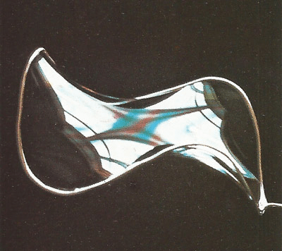
Soap Films
img src: https://www.daviddarling.info/encyclopedia/B/bubbles.html
The Setup
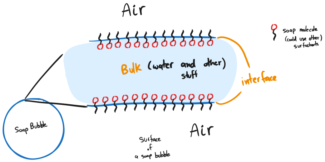
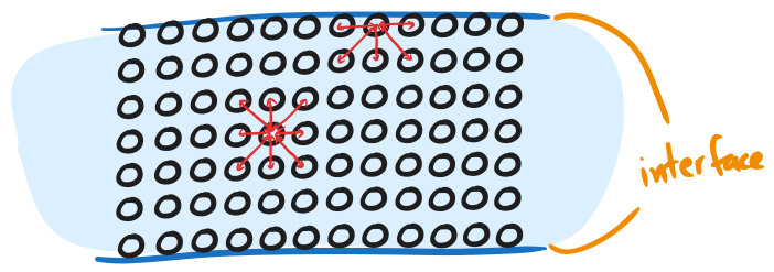
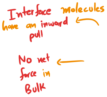
Molecules at the interface have the highest Potential Energy
*the soap film has 2 interfaces
Backup
Soap Interface Force Field
import numpy as np
import matplotlib.pyplot as plt

# y = -1 is the bottom air interface; y = 0 is the center of the bulk liquid; y = 1 is the top air interface
y_points = np.linspace(-1.1, 1.1, 23)
x_points = np.linspace(-1, 1, 9)
X, Y = np.meshgrid(x_points, y_points)

# Define the Force Field
# The force always points towards the bulk (y=0)
# Above the center (y > 0), force is negative (pointing down)
# Below the center (y < 0), force is positive (pointing up)
# At the center (y = 0), force is zero.
F_y = -Y
F_x = np.zeros_like(X) # for visualization, I scale the arrows down

# Mask forces outside the soap film for visual clarity (air has no cohesive pull)
mask = (Y >= -1) & (Y <= 1)
F_y_film = np.where(mask, F_y, 0)
F_y_film *= 0.2

# Define Potential Energy (U): Integrating F_y = -y gives U(y) = 0.5 * y^2
y_curve = np.linspace(-1, 1, 200)
U = 0.5 * y_curve**2

# Create the visualization
fig, (ax1, ax2) = plt.subplots(1, 2, figsize=(12, 6), sharey=True)

# Left Plot: Force Field Vector Map
ax1.quiver(X, Y, F_x, F_y_film, color='crimson', pivot='middle', scale=5)
ax1.set_title('Net Force Field (F)')
ax1.set_xlabel('Horizontal Position')
ax1.set_ylabel('Depth (-1 = Bottom Interface, 0 = Bulk, 1 = Top Interface)')
ax1.set_xlim(-1.2, 1.2)
ax1.set_ylim(-1.2, 1.2)

# Add boundaries for the interfaces and the bulk center
ax1.axhline(0, color='blue', linestyle='--', alpha=0.5, label='Bulk Center (F=0)')
ax1.axhline(1, color='lightblue', linestyle='-', linewidth=4, alpha=0.6, label='Top Air Interface')
ax1.axhline(-1, color='lightblue', linestyle='-', linewidth=4, alpha=0.6, label='Bottom Air Interface')
ax1.legend(loc='upper left', fontsize='small')

# Right Plot: The Potential Well
# Plotted sideways so the Y-axis maps directly to the physical depth of the film
ax2.plot(U, y_curve, color='purple', linewidth=3)
ax2.fill_betweenx(y_curve, 0, U, color='purple', alpha=0.2)
ax2.set_title('Potential Energy Well (U)')
ax2.set_xlabel('Stored Energy (U > 0)')
ax2.set_xlim(0, 0.6)
ax2.grid(True, alpha=0.3)

plt.suptitle('Soap Film as a Potential Well: Two Interfaces and a Central Bulk', fontsize=14)
plt.tight_layout()
plt.show()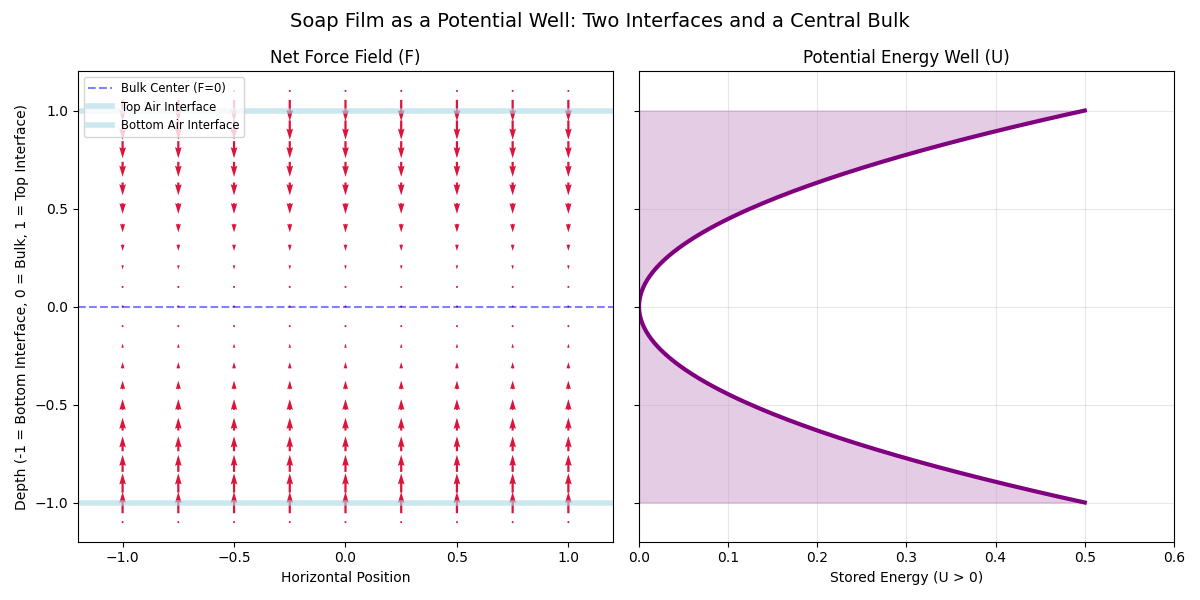
*the soap film has 2 interfaces
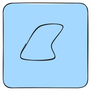
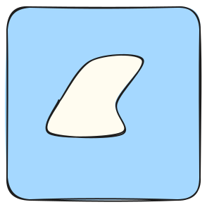
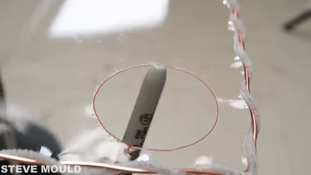
- Thread has a fixed length
- Larger the hole, the smaller the Area of the Soap film
- Fixed Perimeter
- Maximize the Area
Isoperimetric Inequality
Source: How to make inverted bubbles by Steve Mould
How we'll prove it
only true for a circle
area is bounded for all shapes
1.
2.
Let C be a simple closed plane curve with length L, and let A be the area of the region bounded by C. Then
1.
Isoperimetric Inequality
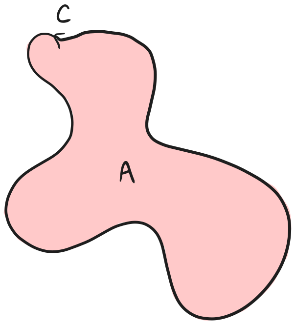
plane curve
closed
simple
Let C be a simple closed plane curve with length L, and let A be the area of the region bounded by C. Then
1.
Isoperimetric Inequality
arc length
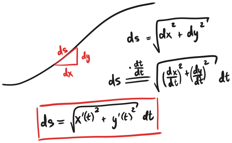
For a curve parameterized by arc length:
What even is the Length of a curve?
Let C be a simple closed plane curve with length L, and let A be the area of the region bounded by C. Then
1.
Isoperimetric Inequality
What even is the Area of a curve?
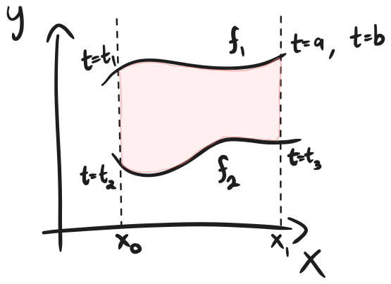
Let C be a simple closed plane curve with length L, and let A be the area of the region bounded by C. Then
1.
Isoperimetric Inequality
What even is the Area of a curve?
A cleaner way is to use Green's Theorem*
only true for a circle
Let C be a simple closed plane curve with length L, and let A be the area of the region bounded by C. Then
1.
2.
Isoperimetric Inequality
What even is the Area of a curve?
Green's Theorem
We want something that connects closed loop curves to 2D integrals:
two simple cases that satisfy that
1.
Isoperimetric Inequality
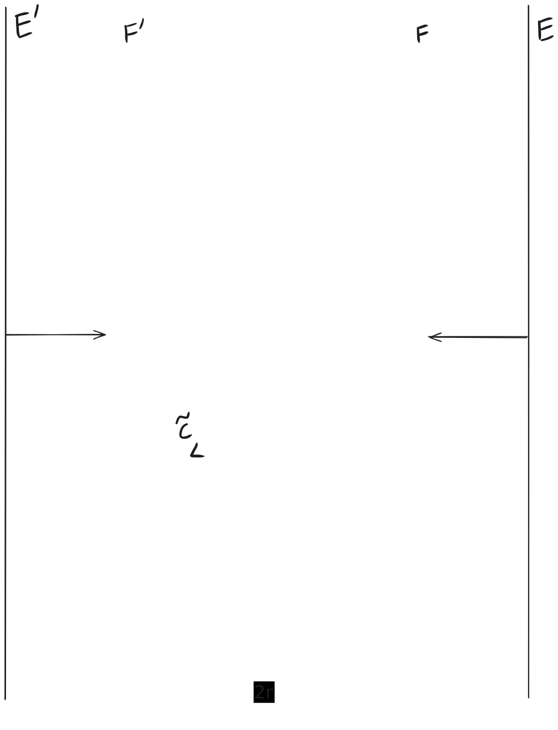
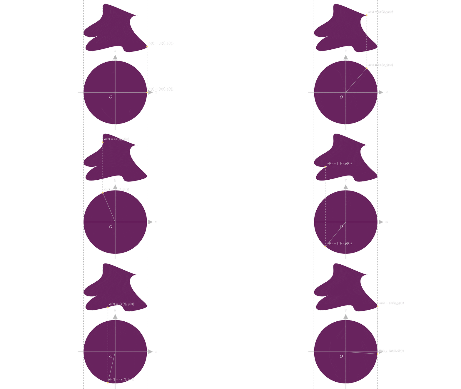
Let C be parameterized by the arc length s , defined
The auxilary circle shares the parameter and function x(t)
Let C be a simple closed plane curve with length L, and let A be the area of the region bounded by C. Then
1.
Isoperimetric Inequality
Let C be a simple closed plane curve with length L, and let A be the area of the region bounded by C. Then
1.
Isoperimetric Inequality
Let C be parameterized by the arc length s
The auxilary circle shares the parameter and function x(t)
Let C be a simple closed plane curve with length L, and let A be the area of the region bounded by C. Then
square both sides
only true for a circle
1.
2.
Isoperimetric Inequality
Let C be a simple closed plane curve with length L, and let A be the area of the region bounded by C. Then
square
solve quadratic
AM-GM property
equality iff x=y
OR
only true for a circle
1.
2.
Isoperimetric Inequality
By coordinate symmetry
this condition is forced for the curve for which the equality holds
References
Differential Geometry of Curves and Surfaces by Manfredo P. do Carmo
How to make inverted bubbles by Steve Mould
https://math.stackexchange.com/questions/19997/a-proof-of-the-isoperimetric-inequality-how-does-it-work
(for additional insights)