PHC6194 SPATIAL EPIDEMIOLOGY

Disease Mapping
Hui Hu Ph.D.
Department of Epidemiology
College of Public Health and Health Professions & College of Medicine
February 21, 2018
Smoothing
Interpolation
Lab: Disease Mapping
Smoothing
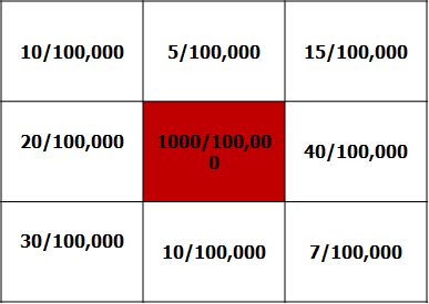
Small Number Issue
- Disease mapping may obscure the spatial pattern of risk
- high rate may be artificially elevated and only reflect lack of data rather than true risk
Two Common Methods to Deal with Small Number Issue
- Probability map
- instead of mapping the disease rates directly, plotting the probability of being more extreme than the observed count in each area under constant risk hypothesis
- Smoothed disease rates
- to borrow information from neighboring areas to produce better (i.e. more stable and less noisy) estimate of the rate associated with an area and thus separate out the "signal" (spatial pattern) from the noise
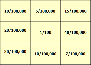
Probability Map
- Assuming disease counts y1, y2, y3, ..., yi follow Poisson distribution
- Under constant risk hypothesis, the overall mean risk is
- The expected case count in area i is:
- We can then calculate the probabilities:

r={{\sum^n_{i=1}y_i} \over {\sum^n_{i=1}n_i}}
\hat E = n_i \times r
Pr(y_i \geq Y_i|E(Y_i)=\hat{E_i})
Pr(y_i \leq Y_i|E(Y_i)=\hat{E_i})
Probability Map
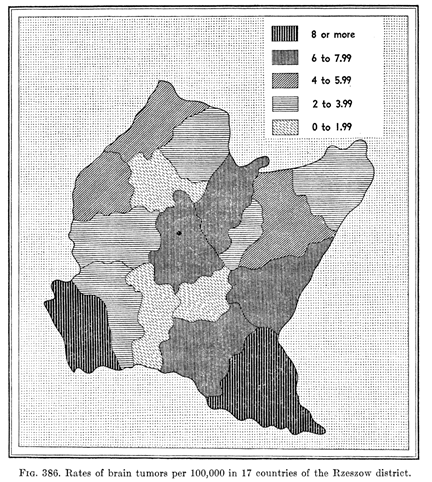
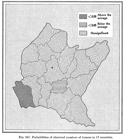
Source: Choynowski , Journal of the American Statistical Association; 1959
- Weakness: The underlying distribution of the data may not agree with the assumption
Smoothing
- Data from locations near one another in space are more likely to be similar than data from locations remote from one another
- How to define neighborhoods
- contiguity: share common boundary
- distance: distance band, KNN
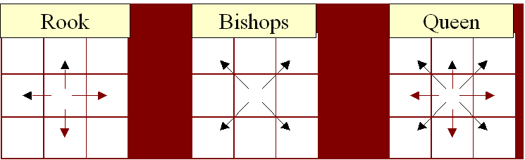
Contiguity
- Rook contiguity:
- polygons that share a border of some length with the current polygon
- Bishops contiguity:
- polygons that shares only a point with the current polygon
- Queen contiguity:
- Rook + Bishops
Distance Band
- Specify a circular smoothing window of specified radius
- Select all neighbors whose centroids are within the smoothing window
KNN
- Choose the k nearest neighbors
Empirical Bayes Smoothing
- Uses Bayesian principles to guide the adjustment of crude rate estimate
- if a crude rate estimate has a small variance (based on a large population at risk), then it will remain essentially unchanged
- Global Empirical Bayes smoothing:
- compromise between the observed rate for the area and an estimate from the entire study area based on probability models
- Local Empirical Bayes smoothing
- compromise between the observed rate for the area and an estimate from a large collection of neighboring areas
- usually requires detailed knowledge of how a study area varies at a small scale
When to Use Smoothing?
- If the addition of one event or one more person at risk results in a large difference in one or more of the rates:
- if a rate change by 25% or more
- If the number of events that forms the numerator of one or more of the rates is less than 3
- If the number of people at risk per region is small
- e.g. <100 people
Strength and Limitations of Smoothing
- Strengths:
- smoothing allows us to stabilize rates based on small numbers by combining available data at the resolution of interest
- reduce noise in the rates caused by different population sizes
- Limitations:
- mapping the rates other than the rates from the raw data
- may introduce other new sources of artifacts
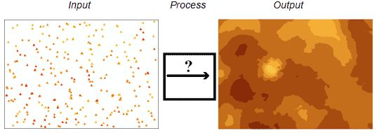
Interpolation
What is Spatial Interpolation
- The procedure of estimating the value at unsampled sites within the area covered by existing samples
Spatial Continuity
- If an observation at a location is similar to other observations nearby
- Or two observations close to each other are more likely to have similar values than two observations that are far apart
- Spatial continuity = positive spatial auto-correlation
- spatial auto-correlation is a correlation of a variable with itself through space
- if nearby or neighboring observations are more alike, this is positive spatial autocorrelation
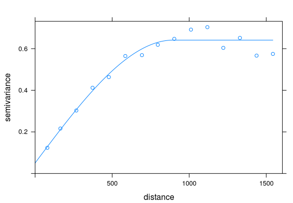
Variogram
- Variogram displays the variances within groups of observations, plotted as a function between the observations
- it is the preferred method for displaying the tendency for nearby observations to be more alike than distant observations
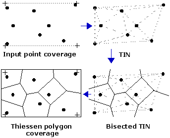
Proximity Interpolation
Nearest Neighbor Interpolation: predict values based on k nearest neighbors
Inverse Distance Weighted Interpolation
- Similar to nearest neighbor interpolation
- The only difference is that points that are further away get less weight in predicting a value of a location
Kriging Interpolation
- The Kriging process fits a theoretical variogram model to a sample variogram of the random variables to guess the underlying random process in the study area
- Then this underlying process is our basis for estimation and evluation
- Ordinary Kriging:
- assumes stationary (a random spatial process is called stationary, if its statistical properties such as mean and variance are independent of absolute location)
- Advantages of Kriging:
- allows adjustment for clustering
- minimizes error and variance
- allows the calculation of 95% CI for each prediction