PHC6194 SPATIAL EPIDEMIOLOGY

Disease Clustering
Hui Hu Ph.D.
Department of Epidemiology
College of Public Health and Health Professions & College of Medicine
February 27, 2019
Introduction
Global Clustering
Local Clustering
Lab: Disease Clustering
Introduction
Spatial Patterns
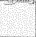
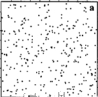
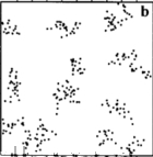
Random
Cluster
Regular
Disease Cluster
- The occurrence of a greater than expected number of cases of a particular disease within a group of people, a geographic area, or a period of time.
- A collection of disease occurrence:
- of sufficient size and concentation to be unlikely to have occurred by chance, or
- related to each other through some social or biological mechanism, or having a common relationship with some other events or circumstance
- Spatial aggregation of disease events may only be a function of the distribution of population
- Disease cluster: residual spatial variation in risk after known influence have been accounted for
Purposes of Disease Cluster Detection
- Confirmatory purpose
- verify if a perceived cluster exists:
e.g. excess risk reported by citizens
- Exploratory purpose
- search for spatial patterns
- Identification of clusters can lead to interventions
Methods of Disease Cluster Detection
- Global clustering:
- non-specific methods
- only detect if cluster exists, without specific location
- Local clustering:
- specific methods
- shows the specific locations where clusters exist
- two methods: non-focused and focused
Global Clustering
Global Clustering (Non-specific Methods)
-
Evaluate whether clustering exist as a global phenomena throughout the study region, without pinpointing the location of specific cluster
- e.g. the analysis of overall clustering tendency of some disease incidence in a study region
Tests for Global Clustering
- Over 100 different testing methods for global clustering in the field
- Some widely-used methods:
- for aggregated data:
Moran's I
Geary's C
- for points data:
KNN
Moran's I
- Moran's I is a global index of spatial auto-correlation
- to quantify the similarity of an variable among areas that are defined as spatially related
- Calculation:
- N: number of spatial units indexed by i and j
- X: the variable of interest
- wij: a matrix of spatial weights
I={{N}\over {\sum_i(X_i-\bar X)^2}}\times {{\sum_i\sum_jw_{ij}(X_i-\bar X)(X_j-\bar X)}\over {\sum_i\sum_jw_{ij}}}
Moran's I (cont'd)
- Moran's I coefficient of auto-correlation is similar to Pearson's correlation coefficient
- I>0
- positive spatial auto-correlation
- neighboring regions tend to have similar values
- I<0
- negative spatial autocorrelation
- neighboring regions tend to have inverse values
- Results will depend on specification of the weight matrix
Geary's C
- Also called Geary's contiguity ratio
- Another widely used global index of spatial auto-correlation
- Calculation:
- N: number of spatial units indexed by i and j
- X: the variable of interest
- wij: a matrix of spatial weights
C={{N-1}\over {2\sum_i(X_i-\bar X)^2}}\times {{\sum_i\sum_jw_{ij}(X_i-X_j)^2}\over {\sum_i\sum_jw_{ij}}}
Geary's C (cont'd)
- Geary's C ranges from 0 to 2
- Low value of Geary's C denote positive auto-correlation
- 0 indicates perfect positive spatial auto-correlation
- High value of Geary's C denote negative auto-correlation
- 2 indicates perfect negative spatial auto-correlation
- 1 indicates no auto-correlation
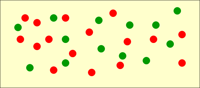
KNN
- Proposed by Cuzick and Edward
- To detect the possible clustering of sub-populations within a clustered or non-uniformly-spread overall population
- Based on the locations of cases and randomly selected controls from a specified region
KNN (cont'd)
- Central idea of the method: to find how many of the K nearest neighbors of a cases that are also cases
- A weight matrix based on KNN
- wij=1 if location j is among k nearest neighbors of location i
- The test statistics:
- 𝛿=1 if the point is a case, 𝛿=0 if the point is a control
T_k=\sum_{i=1}^n \sum_{j=1}^n w_{ij}\delta_i\delta_j
KNN (cont'd)
- Monte Carlo test under the random labeling hypothesis is used to test the significance
- The rank of the test statistic is based on the data observed among the values from the randomly labeled data, which allows calculation of the p-value
Local Clustering
Local Clustering Test
- Additionally specify the location and can be extended to also consider temporal patterns
- Focused tests:
- investigate whether there is an increased risk of disease around a pre-determined point
- e.g. Superfund site; A nuclear power plant; A waste dumping site
- Non-focused tests:
- identify the location of all potential clusters in the study region
Focused Tests
- H0: there is no cluster of cases around the foci
- The Lawson Waller test
- also called Berman's Z1 test
- H0: yi~ Poisson(ni*r)
- H1: yi~ Poisson(ni*r (1+εθi)), where θi represents exposure to the foci experienced by population in region i; ε represents a small, positive constant
- what is the relative risk comparing people in region i with people with no exposure
-
The Lawson Waller score
- where θi is defined by the inverse distance of each region from the foci
- usually standardized to range from 0 to 1
T_{sc}=\sum_{i=1}^N\theta_i(y_i-rn_i)
Non-focused Tests
- Aggregated data:
- Local Indicators of Spatial Auto-correlation (LISA)
- Local Getis-Ord G statistics
- Spatial scan statistics
- Point data:
- Openshaw's Geographical analysis Machine (GAM)
- Turnbull's cluster evaluation permutation procedure (CEPP)
- Spatial scan statistics
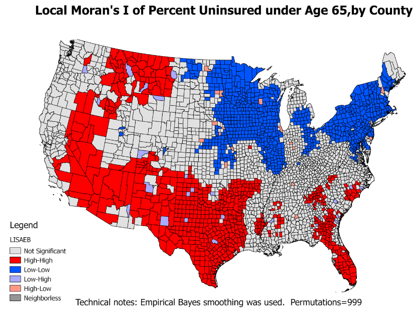
LISA
- Also called Local Moran's I
- LISA values allow for the computation of its similarity with its neighbors and also to test its significance
- LISA divides the study region into 5 categories:
- high-high locations: also known as hot spots
- low-low locations: also known as cold spots
- high-low locations: potential spatial outliers
- low-high locations: potential spatial outliers
- locations with no significant local auto-correlation
Local Getis-Ord G Statistic
- The proportion of all x values in the study area accounted for by the neighbors of location i
- G will be high where high values cluster (hot spot)
- G will be low where low values cluster (cold spot)
G_i(d)={{\sum_jw_{ij}x_j}\over {\sum_jx_j}}
Spatial Scan Statistic
- Steps:
- search over a given set of spatial regions
- find those regions which are most likely to be clusters
- correctly adjust for multiple hypothesis testing
Search Over a Given Set of Spatial Regions
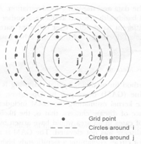
- Create a regular or irregular grid of centroids covering the whole study area
- Create an infinite number of circles around each centroid, with the radius ranging from 0 to a maximum which includes at most 50% of the population
- A circular scanning window is placed at different coordinates with radius that vary from 0 to some set upper limit.
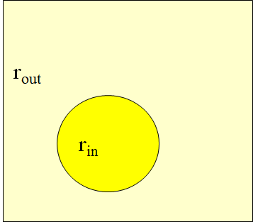
Find Regions that are Most Likely to be Clusters
- For each location and size of window
H = elevated risk within window as compared to outside of window
- Is there any region with disease rates significantly higher inside the circle than outside the circle ?
- For each circle, obtain the actual and expected number of cases inside and outside the circle, and calculate likelihood function
A
Find Regions that are Most Likely to be Clusters (cont'd)
- Generate random replicas of the dataset under the null-hypothesis of no clusters (Monte Carlo sampling)
- Compare most likely clusters in real and random datasets (likelihood ratio test)
Properties of Spatial Scan Statistics
- Adjusts for inhomogeneous population density
- Simultaneously tests for clusters of any size and any location, by using circular windows with continuously variable radius
- Accounts for multiple testing
- Possibility to include confounding variables
- Can be used with both aggregated and point data