PHC6937 Public Health Research Methods

Machine Learning
Hui Hu Ph.D.
Department of Epidemiology
College of Public Health and Health Professions & College of Medicine
huihu@ufl.edu
April 9, 2020
Introduction
Bias-Variance Trade-off
Regularization
Decision Trees and Ensembles
Neural Networks and Deep Learning
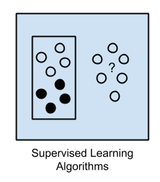
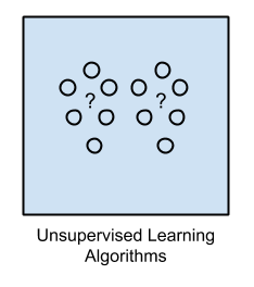
Introduction
Inferential Model
vs
Predictive Model
The Limits of Traditional Computer Programs
Image from MNIST handwritten digit dataset
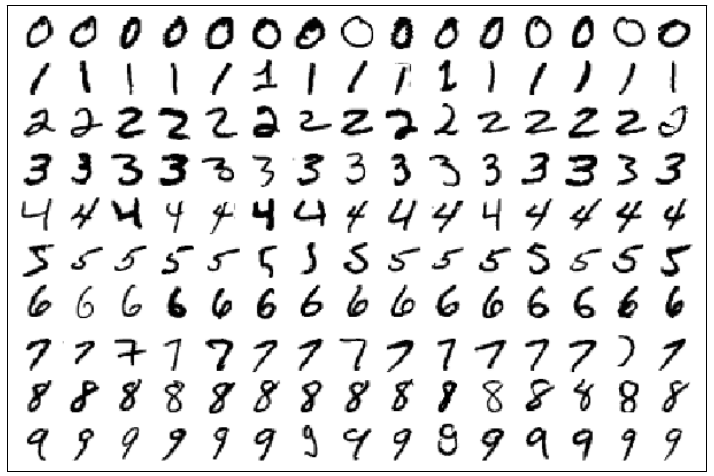
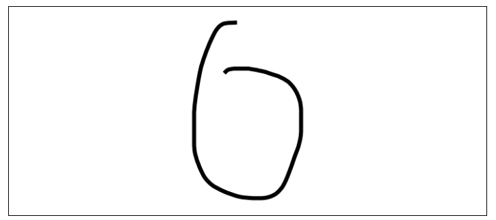
A zero that is difficult to distinguish from a six algorithmically
- How to distinguish between threes and fives?
- Or between fours and nines?
We don't know what program to write because we don't know how it's done by our brains
Machine Learning
- Many things we learn in school have a lot in common with traditional computer programs:
how to multiply numbers, solve equations, take derivatives
- The things we learn at an extremely early age, the things we find most natural, are learned by example, not by formula:
recognize a dog
- In other words, when we were born, our brains provided us with a model that described how we would be able to see the world
- as we grew up, that model would take in our sensory inputs and make a guess about what we're experiencing
- if that guess is confirmed by our parents, our model would be reinforced
- over our lifetime, our model becomes more and more accurate as we assimilate billions of examples
Machine Learning
- Machine learning is predicated on this idea of learning from example
- Instead of teaching a computer a massive list rules to solve the problem, we give it a model with which it can evaluate examples and a small set of instructions to modify the model when it makes a mistake

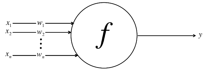
Let's define our model to be a function
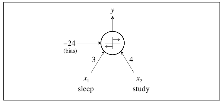
Another Example
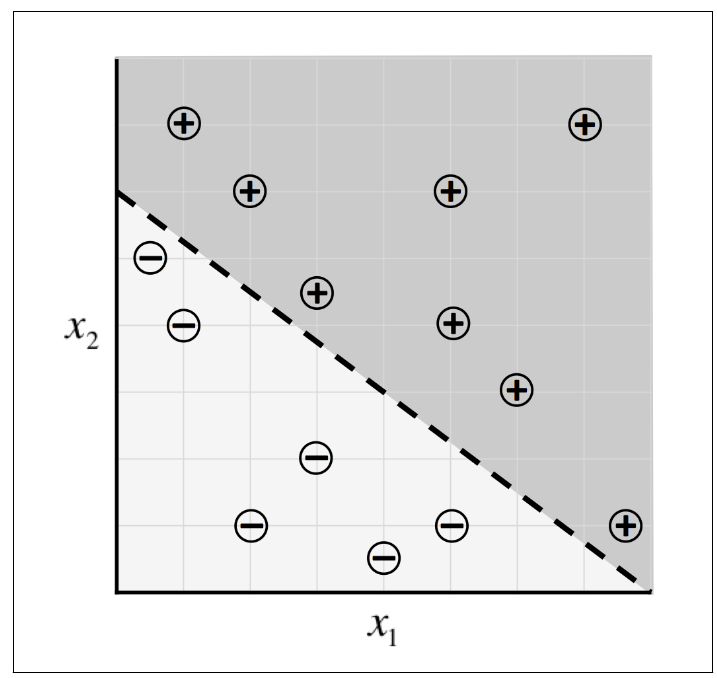
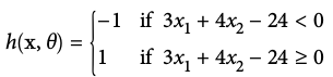
- To predict exam performance (above or below average) based on the number of hours of sleep we get and the number of hours we study in the previous day
- We collect a lot of data
- Our goal might be to learn a model with parameter vector
such that:
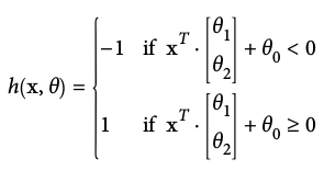
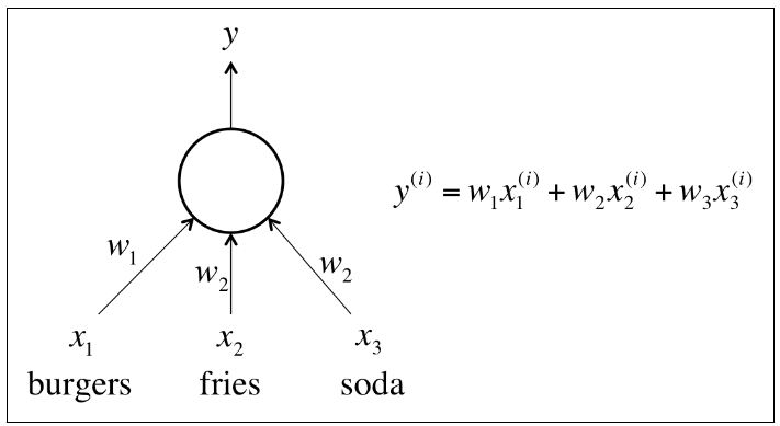
A linear perceptron
Deep Learning
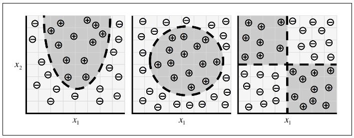
- As we move on to much complex problems, our data
- not only becomes extremely high dimensional
- the relationships we want to capture also become highly nonlinear
- To accommodate this complexity, recent research in machine learning has attempted to build models that highly resemble the structures utilized by our brains
- Commonly referred to as deep learning, which has had spectacular success in tackling problems in computer vision and natural language processing
- not only far surpass other kinds of machine learning algorithm
- also rival the accuracies achieved by humans
Bias-Variance Trade-off
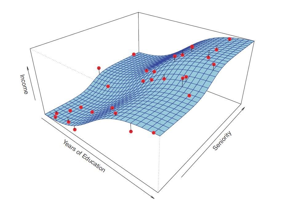
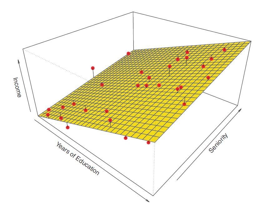
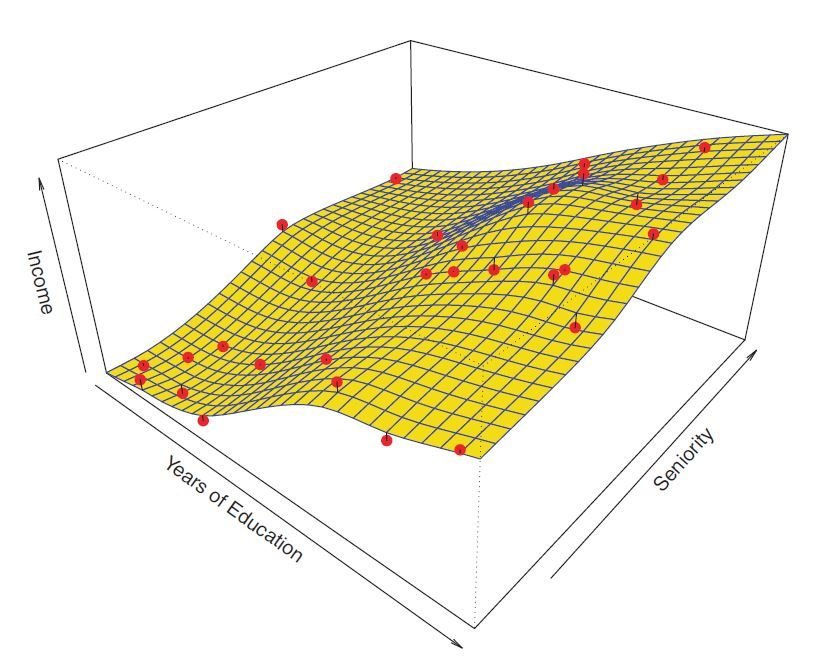
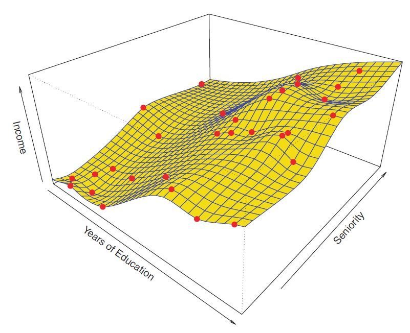
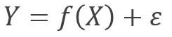
Decomposition of Error
- The underlying relationship between X and Y:
- We usually estimate f() for two reasons:
- prediction
- inference - The prediction model:
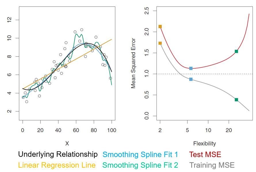
- We can decompose the squared difference between the predicted value and the actual value of Y:
- reducible error:
- irreducible error: - We aim to generate models that can minimize the reducible error.


Bias-Variance Trade-off
Cross-Validation
- The test error can be calculated if a test dataset is available.
- Unfortunately, this is usually not the case.
We don’t have a very large designated test dataset that can be used to directly estimate the test error in most time.
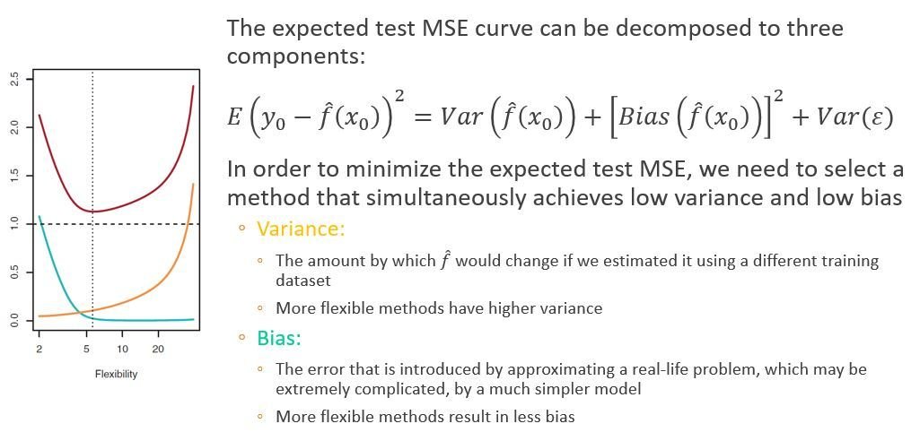
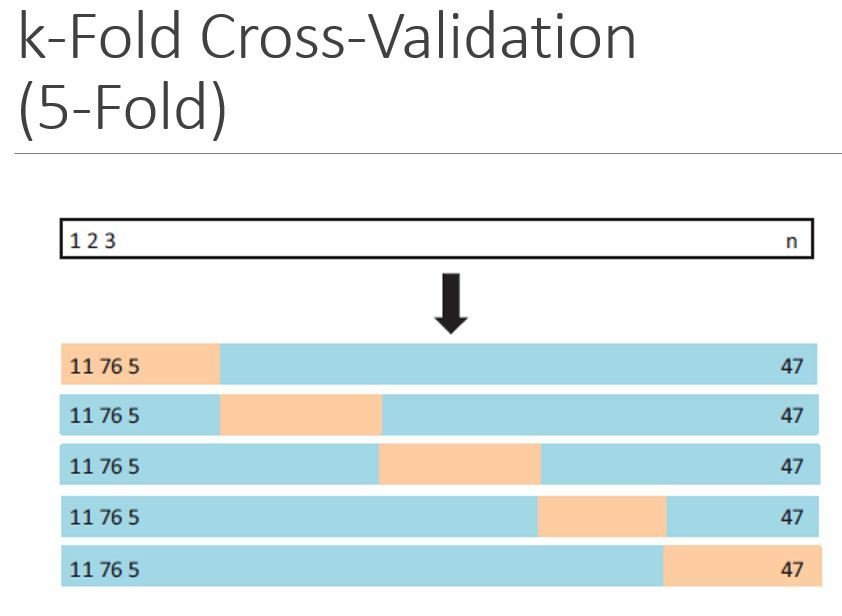
- Cross-validation:
A method that can estimate the test error by holding out a subset of the training observations from the fitting process, and then applying the trained method to those held out observations
Training
80%
Testing
20%
k-fold CV
Tune Models
Evaluate Performance
Raw Data
Data Engineering
Explore
Model Selection
Feature Engineering
Train Model
Evaluate Performance
Data Product
Machine Learning Pipeline
Regularization
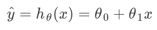
Linear Regression with One Variable
The hypothesis function:
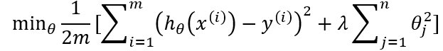
Cost function:
- measures the accuracy of our hypothesis function by using a cost function.
- takes an average of all the results of the hypothesis with inputs from x's compared to the actual output y's
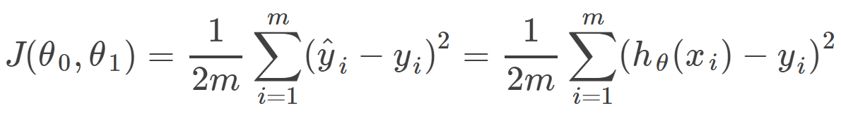
- This function is otherwise called the "Squared error function", or "Mean squared error".
- The mean is halved as a convenience for the computation of the gradient descent, as the derivative term of the square function will cancel out the 1/2 term.
Gradient Descent
Now we need to estimate the parameters in hypothesis function.

- The way we do this is by taking the derivative of our cost function.
- The slope of the tangent is the derivative at that point and it will give us a direction to move towards.
- We make steps down the cost function in the direction with the steepest descent, and the size of each step is determined by the parameter α, which is called the learning rate.
Gradient Descent
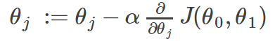
The gradient descent algorithm is:
repeat until convergence:
where j=0,1 represents the feature index number.
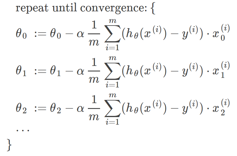
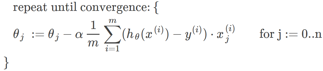
Gradient Descent for Linear Regression:
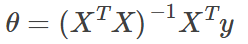
Why Gradient Descent?
Normal Equation:
| Gradient Descent | Normal Equation |
|---|---|
| Need to choose alpha | No need to choose alpha |
| Needs many iterations | No need to iterate |
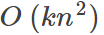
| Works well when n is large |
Slow if n is very large |

For large datasets, we usually use stochastic gradient descent.
Regularization
-
High bias or underfitting:
- when the form of our hypothesis function maps poorly to the trend of the data.
- It is usually caused by a function that is too simple or uses too few features. -
High variance or overfitting:
- caused by a hypothesis function that fits the available data well but does not generalize well to predict new data.
- It is usually caused by a complicated function that creates a lot of unnecessary curves and angles unrelated to the data. -
Two main options to address overfitting:
- Reduce the number of features (manually select which features to keep/use a model selection algorithm)
- Regularization (Keep all the features, but reduce the parameters θ)
Regularization
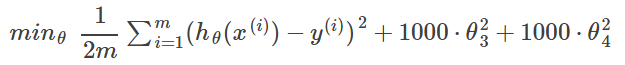
If we have overfitting from our hypothesis function, we can reduce the weight that some of the terms in our function carry by increasing their cost.
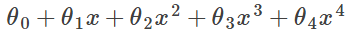
We want to make it more quadratic
We'll want to eliminate the influence of the cubic and quartic terms.
Without actually getting rid of these features or changing the form of our hypothesis, we can instead modify our cost function:
In general:
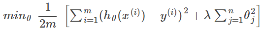
L2 regularization (Ridge)
Regularization
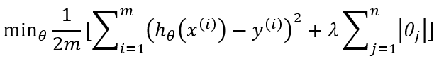
L1 regularization (Lasso):
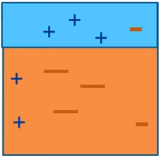
L2 regularization (Ridge):
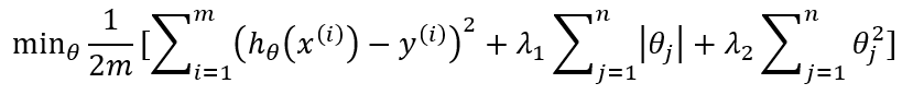
L1+L2 regularizations (Elastic net):
Comparisons
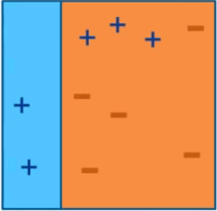
- L1 regularization helps perform feature selection in sparse feature spaces
- L1 rarely perform better than L2
- when two predictors are highly correlated, L1 regularizer will simply pick one of the two predictors
- in contrast, the L2 regularizer will keep both of them and jointly shrink the corresponding coefficients a little bit
- Elastic net has proved to be (in theory and in practice) better than L1/Lasso
Decision Trees and Ensembles
- Modern name: Classification and Regression Trees (CART)
- The CART algorithm provides a foundation for important algorithms such as bagged decision trees, random forests, and boosted decision trees
CART Model Representation
- Binary tree
- Node: a single input variable (x) and a split point on that variable
- Leaf node: an output variable (y)
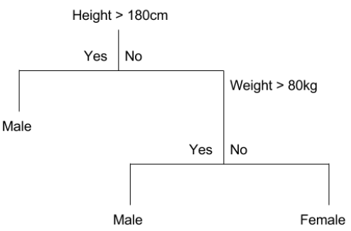
Making Predictions
- Evaluate the specific input started at the root node of the tree
- Partitioning of the input space
- e.g. height=160cm, weight=65kg
- Height>180cm: No
- Weight>80kg: No
- Therefore: Female
Learn a CART Model from Data
- Creating a binary decision tree is actually a process of dividing up the input space
- A greedy approach is used: recursive binary splitting
- all the values are lined up and different split points are tried and tested using a cost function
- the split with the best cost is selected
- Cost functions:
- regression: the sum of squared error
- classification: the Gini cost
Stopping Criterion
- The recursive binary splitting procedure needs to know when to stop splitting as it works its way down the tree with the training data
- Most common stopping procedure:
- set a minimum count on the number of training instances assigned to each leaf node
- defines how specific to the training data the tree will be
- too specific (e.g. 1) will lead to overfit
- needs to be tuned
Pruning the Tree
- Pruning can be used after the tree is learned to further lift performance
- The complexity of a decision tree is defined as the number of splits in the tree
- Simple trees are preferred
- easy to understand
- less likely to overfit your data
- Work through each leaf node in the tree and evaluate the effect of removing it
- leaf nodes are removed only if it results in a drop in the overall cost function
- Ensembles (combine models) can give you a boost in prediction accuracy
- Three most popular ensemble methods:
- Bagging: build multiple models (usually the same type) from different subsamples of the training dataset
- Boosting: build multiple models (usually the same type) each of which learns to fix the prediction errors of a prior model in the sequence of models
- Voting: build multiple models (usually different types) and simple statistics (e.g. mean) are used to combine predictions
Ensembles
Bagging
- Take multiple samples from your training dataset (with replacement) and train a model for each sample
- The final output prediction is averaged across the predictions of all of the sub-models
- Performs best with algorithms that have high variance (e.g. decision trees)
- Run in parallel because each bootstrap sample does not depend on others
- Common algorithms:
- bagged decision trees
- random forest
with reduced correlation between individual classifiers
a random subset of features are considered for each split
- extra trees
further reduce correlation between individual classifiers
cut-point is selected fully at random, independently of the outcome
Bootstrap Aggregation
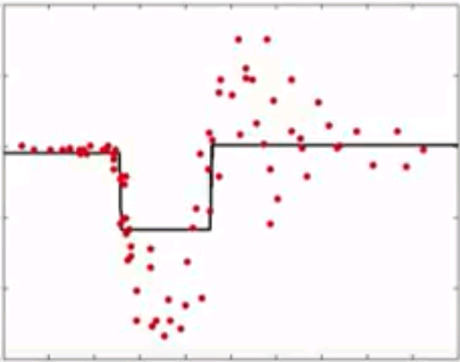
Boosting
- Creates a sequence of models that attempt to correct the mistakes of the models before them in the sequence
-
Build a model from the training data, then create a second model that attempts to correct the errors from the first model
-
Once created, the models make predictions which may be weighted by their demonstrated accuracy and the results are combined to create a final output prediction
-
Models are added until the training set is predicted perfectly or a maximum number of models are added
- Works in sequential manner
Common Algorithms
AdaBoost (Adaptive Boosting)
- Weight instances in the dataset by how easy or difficult they are to predict
-
Allow the algorithm to pay more or less attention to them in the construction of subsequent models
Gradient Boosting (Stochastic Gradient Boosting)
- Boosting algorithms as iterative functional gradient descent algorithms
- At each iteration of the algorithm, a base learner is fit on a subsample of the training set drawn at random without replacement
AdaBoost (Adaptive Boosting)
- Initialize observation weights:
- For m=1 to M
- fit a classifier Gm(x) to training data
- compute:
- compute:
- set:
AdaBoost (Adaptive Boosting)

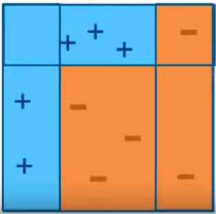
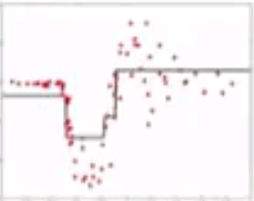
Iteration 1
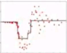
Iteration 2
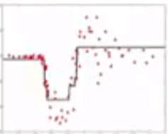
Iteration 3
Final Model
Intuitive sense: weights will be increased for incorrectly classified observation
- give more focus to next iteration
- weights will be reduced for correctly classified observation
Gradient Boosting
- Instead of reweighting observations in adaptive boosting, gradient boosting make some corrections to prediction errors directly
- Learn a model -> compute the error residual -> learn to predict the residual
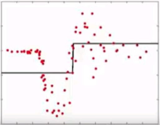
Initial model
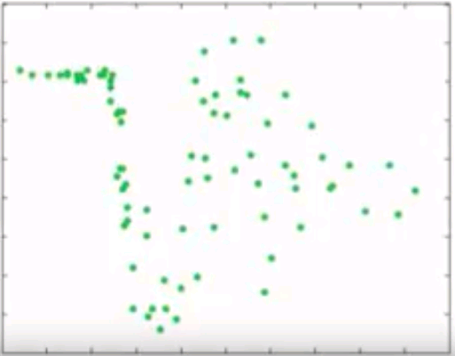
Compute residuals
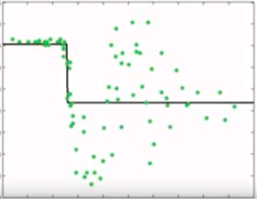
Model residuals
Combinations
...
Gradient Boosting
- Learn sequence of models
- Combination of models is increasingly accurate and increasingly complex
Model predictions
Residuals
...
Neural Networks and
Deep Learning
Neural Networks
- A field of study that investigates how simple models of biological brains can be used to solve difficult computational tasks (i.e. predictive modeling in machine learning)
- the goal is not to create realistic model of the brain
- develop robust algorithms and data structures that can be used to model difficult problems
- NNs are capable of learning any mapping function and have been proven to be a universal approximation algorithm
- the predictive capability of NNs comes from the hierarchical/multilayered structure of the networks
- the data structure can pick out features at different scales or resolutions and combine them into higher-order features
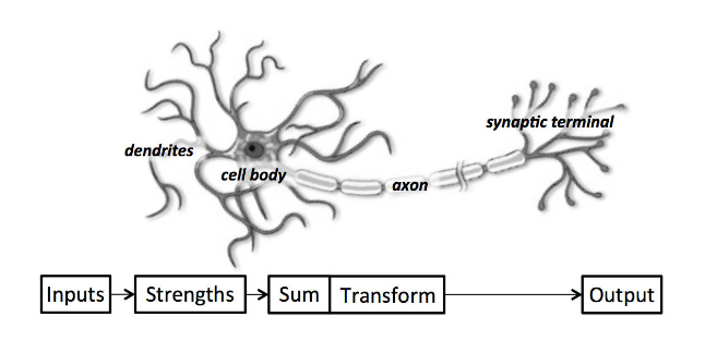
Perceptron
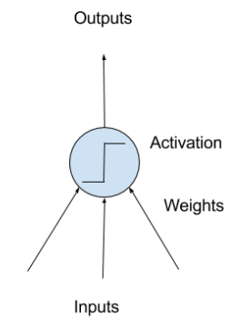
- Perceptron:
- a single neuron model that was a precursor to larger neural networks
- neuron
- neuron weights
- activation
- Neuron: the building block for NNs
- simple computational units that have weighted input signals and produce an output signal using an activation function
Perceptron
- Neuron weights:
- similar to the coefficients used in a regression equation
- like linear regression, each neuron also has a bias which can be thought of as an input that always has the value 1.0 and it too must be weighted (e.g. a neuron may have 2 inputs, and it requires 3 weights)
- weights are often initialized to small random values (i.e. 0~0.3)
- Activation:
- the weighted inputs are summed and passed through an activation function (also called a transfer function)
- it governs the threshold at which the neuron is activated and the strength of the output signal
- historically, simple step activation functions were used (e.g. if the summed input was above a threshold, say 0, then the neuron would output a value of 1, otherwise, output a -1)
Expressing Linear Perceptrons
Feed-forward Neural Networks
- Single neurons are not expressive enough to solve complicated learning problems
- The neurons in the human brain are organized in layers
- information flows from one layer to another
- sensory input is converted into conceptual understanding

Feed-forward NNs:
- connections only traverse from a lower layer to a higher layer
- no connections between neurons in the same layer
- no connections that transmit data from a higher layer to a lower layer
Linear Activation

- Linear activation is easy to compute with, but has serious limitations
- Any feed-forward NN consisting of only linear activation can be expressed as a NN with no hidden layers
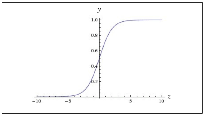
Nonlinear Activation
- In order to learn complex relationships, we need to use activation functions that employ some sort of nonlinearity
Logistic function / Sigmoid function: 0~1
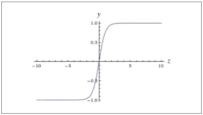
Hyperbolic tangent (Tanh) function: -1~1
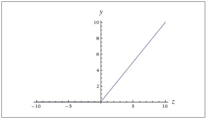
ReLU (rectified linear unit) function
Networks of Neurons
- Neurons are arranged into networks of neurons:
- a row of neurons is called a layer
- the architecture of the neurons in the network is often called the network topology
- Input or Visible Layer:
- the bottom layer, which takes input from the dataset
- usually with one neuron per feature in the dataset
- Hidden Layers:
- not directly exposed to the input
- the simplest network structure is to have a single neuron in the hidden layer that directly outputs the value
- deep learning can refer to having many hidden layers in NN
- Output Layer:
- the final hidden layer
- the choice of activation function in the output layer is constrained by the type of problem that you are modeling
- e.g. single output neuron with no activation function for regression problem, single output neuron with a sigmoid function for binary classification problem, softmax output layer for multiclass classification problem

Training Networks
- Data Preparation:
- data must be numerical (one-hot encoding for categorical features)
- NNs require the input to be scaled in a consistent way (e.g. normalization)
-
Stochastic Gradient Descent:
- classical training algorithm for NNs
- one row of data is exposed to the network at a time as input
- the network processes the input upward activating neurons as it goes to finally produce an output value (forward propagation)
- the output of the network is compared with the expected output and an error is calculated
- this error is then propagated back through the network, one layer at a time, and the weights are updated according to the amount that they contributed to the error (back propagation algorithm)
- the process is repeated for all of the examples in training data
- one round of updating the network for the entire training dataset is called an epoch
Prediction
- Once a NN has been trained, it can be used to make predictions
- The network topology and the final set of weights is all that you need to save from the model
- Predictions are made by providing the input features to the network and performing a forward-pass allowing it to generate an output that you can use as a prediction
Convolutional Neural Network
- The flattening of the image matrix of pixels to a long vector of pixel values looses all of the spatial structure in the image
C
C
C
C
C
-'C'
-'C'
-'C'
-'C'
-?
Does color matter?
No, only the structure matters
- Preserve the spatial relationship between pixels by learning internal feature representations using small squares of input data
- Features are learned and used across the whole image
- allowing for the objects in the images to be shifted or translated in the scene and still detectable by the network
- Advantages of CNNs:
- fewer parameters to learn than a fully connected network
- designed to be invariant to object position and distortion in the scene
- automatically learn and generalize features from the input domain
CNN
Building Blocks of CNNs

Recurrent Neural Network
Sequences
- Time-series data:
- e.g. price of a stock over time
- Classical feedforward NN:
- define a window size (e.g. 5)
- train the network to learn to make short term predictions from the fixed sized window of inputs
- limitations: how to determine the window size
- Different types of sequence problems:
- one-to-many: sequence output, for image captioning
- many-to-one: sequence input, for sentiment classification
- many-to-many: sequence in and out, for machine translation
- synchronized many to many: synced sequences in and out, for video classification
RNNs
- RNNs are a special type of NN designed for sequence problems
- A RNN can be thought of as the addition of loops to the archetecture of a standard feedforward NN
- the output of the network may feedback as an input to the network with the next input vector, and so on
- The recurrent connections add state or memory to the network and allow it to learn broader abstractions from the input sequences
Reading