Motion Planning for Planar Pushing with Convex Optimization
Long Talk, RLG MIT
December 8th 2023
Bernhard Paus Graesdal
Note
- This is pretty much how I am planning to structure/present the material in the paper
- Feedback is much appreciated!
- I have tried to keep notation clean - let me know when it is not!
Agenda
- SPP in graphs of convex sets
- Planning through contact as a SPP
- Semidefinite relaxations of QCQPs
- SPP in graphs of basic semi-algebraic sets
- Mechanics of planar pushing
- Results
- Discussion & future work
Motivation
C. Chi et al., “Diffusion Policy: Visuomotor Policy Learning via Action Diffusion.” Mar. 09, 2023
- Not currently a good solution to planning...
- ...mode sequence and trajectories within modes simultaneously
- ...contact locations, contact forces, and object poses simultaneously
- We will try to address these problems
A quick look at some recent papers
N. Doshi, F. R. Hogan, and A. Rodriguez, “Hybrid Differential Dynamic Programming for Planar Manipulation Primitives,” 2020
T. Lefebvre, S. De Witte, T. Neve, and G. Crevecoeur, “Differential Flatness of Slider-Pusher Systems for Constrained Time Optimal Collision Free Path Planning.” 2023
- Able to switch contact sequence
- Fixed contact positions
- One contact mode only
- Not able to constrain slider orientation
J. Zhou and M. T. Mason, “Pushing revisited: Differential flatness, trajectory planning and stabilization” 2019
- Fixed contact point
- One contact mode only
- (not able to constrain slider orientation?)
SPP in Graphs of Convex Sets (1/2)
- Given a vertex set \( \mathcal{V} \) and an edge set \( \mathcal{E} \subset \mathcal{V}^2\), let \(G = (\mathcal{V},\mathcal{E})\) be a directed graph
- Given compact convex sets \( \mathcal{X}_v \subset \R^{N_v}\) and an associated point \( x_v \in \mathcal{X}_v\) for each \(v\in\mathcal{V}\)
- Source and target vertices \( s, t \in \mathcal{V} \)
- Convex edge costs \[l_e: \R^{N_u} \times \R^{N_v} \rightarrow \R, \; l_e(x_u, x_v) \geq 0 \]
- Convex edge sets \( \mathcal{X}_e \subset \R^{N_u} \times \R^{N_v}, \, e = (u,v)\)
SPP in Graphs of Convex Sets (2/2)
- Let \( \mathcal{P} \) be the set of all \(s\)-\(t\) paths in \( G \), and \( \mathcal{E}_p \) the set of edges traversed by a path \( p \in P \)
- The SPP in a graph of convex sets can then be formulated as:
T. Marcucci, J. Umenberger, P. A. Parrilo, and R. Tedrake, “Shortest Paths in Graphs of Convex Sets.” arXiv, Sep. 21, 2022.
Planning Through Contact as a SPP (1/5)
- Let \(\mathcal{M}\) be a set of contact modes
- Let \(\mathcal{T} \subset \mathcal{M}^2\) be a set of allowable mode transitions
-
Let \(x\in \R^{N_x}\) and \(u\in\R^{N_u}\) represent the state and input of the system
- With \(m \in \mathcal{M}\) associate a trajectory segment defined as a finite sequence of \(N_m\) state-input pairs \[(x_k, u_k) \in \R^{N_x+N_u}, \, k = 1, \ldots, N_m\]
- Represented by the vector \[\xi_m = ((x_0, u_0), \ldots, (x_{N_m}, u_{N_m})) \in (\R^{N_x+N_u})^{N_m}\]
For a given system:
- Associate a cost function \(l_m: (\R^{N_x+N_u})^{N_m} \rightarrow \R\)
- s.t. \(l_m(\xi_m) \in \R \) and \( l_m \) polynomial
- Associate explicit (or implicit) dynamics represented by \[f_m: \R^{N_x}\times\R^{N_u} \rightarrow \R^{N_x} \quad \text{s.t.} \quad x_{k+1} = f_m(x_k, u_k), \, k = 1, \ldots, N_m - 1\]
- Implicit case: \[g_m: \R^{N_x}\times\R^{N_x}\times\R^{N_u} \rightarrow \R^{M} \quad \text{s.t.} \quad g_m(x_k, x_{k+1}, u_k) = 0, \, k = 1, \ldots, N_m - 1\]
- \( f_m, \, g_m \) polynomial
Planning Through Contact as a SPP (2/5)
For each \(m\in\mathcal{M}\):
State and input constraints for each \(m\in\mathcal{M}\):
-
Polynomial state constraints, represented by the basic semi-algebraic set \[\mathcal{X}_m = \set{x \in \R^{N_x} \mid p_1(x) \geq 0, \ldots, p_{L_m}(0) \geq 0}\] where \(p_i, \, i = 1, \ldots, L_m\) are polynomials in \(x\)
-
Linear input constraints represented by the polyhedron \(\mathcal{U}_m \subset \R^{N_u}\)
Planning Through Contact as a SPP (2/5)
- The set of all valid trajectory segments \(\xi_m\) for \(m\) then given as:
Where \(\mathcal{Z}_m\) is a basic semi-algebraic set
Planning Through Contact as a SPP (3/5)
(or equivalently in the implicit dynamics case)
- For all mode transitions \((m, n) \in \mathcal{T} \) define \[ \mathcal{C}_{(m,n)} = \set{(\xi_m, \xi_n) \mid x^{(m)}_{N_m} = x^{(n)}_{0}} \] as the set of all trajectory segments \(\xi_m\) and \(\xi_n\) where the state is constant in the transition between modes
- \((\mathcal{M}, \mathcal{T})\), \(\xi_m \in \mathcal{Z_m}\) for each \(m \in \mathcal{M}\) now defines a graph of basic semi-algebraic sets
- (with \(\mathcal{C}_{(m,n)} \) for each \((m,n) \in \mathcal{T}\) being edge constraints)
Planning Through Contact as a SPP (3/5)
Given a starting and end mode \(s, t \in \mathcal{M}\):
- Define an \(s\)-\(t\) path \(p\) as a finite sequence of distinct modes \((m_0, \ldots, m_K)\) such that \(m_0 = s\) and \(m_K = t\), and \((m_k, m_{k+1}) \in \mathcal{T}\) for all \(k = 0, \ldots, K\).
- Let \(\mathcal{P}\) be the set of all \(s\)-\(t\) paths given \(\mathcal{M}\) and \(\mathcal{T}\)
Planning Through Contact as a SPP (4/5)
Now, we can state the motion planning through contact problem as the following SPP in a graph of basic-semialgebraic sets
The decision variables are the discrete path \(p\) and the continuous variables \(\xi_m\).
Intuition:
Planning Through Contact as a SPP (5/5)
Note: This is almost a SPP in GCS problem, except for non-convex sets
Basic Semi-Algebraic sets \(\rightarrow\) Quadratic Constraints
- Let \( x \in \R^N \)
- Given a basic semi-algebraic set:
- \(\mathcal{S} = \set{x \in \R^{N} \mid p_1(x) \geq 0, \ldots, p_{K}(0) \geq 0}\), where \(p_i, \, i = 1, \ldots, K\) are polynomials in \(x\)
- By introducing lifting variables, \(\mathcal{S}\) can be described by only degree 2 polynomials
- Example:
- Consider the variety in \(\R^2\) given by \(x^2y = 0 \).
- Introduce \(z=x^2\)
- The variety can now be described in \(\R^3\) by \( zy=0\) and \(z = x^2\)
- Given a QCQP in homogenuous form:
- \(x \in \mathbb{R}^{n+1}\), \(y \in \mathbb{R}^n\), \(A \in \mathbb{R}^{m \times (n+1)}\), and \(Q_i \in \mathbb{R}^{(n+1) \times (n+1)}, \, i = 0, \ldots, l\).
- Note: positive-semidefiniteness is not required for \(Q_i, \, i=0, \ldots, l\), hence the problem can be non-convex and in general NP-hard
Semidefinite Relaxations of QCQPs (1/5)
- Using \(x^\intercal Q_i x = \text{tr}(Q_i x x ^\intercal)\) and substituting \(X = xx^\intercal\) we equivalently write:
- \(e_1\) is the \((n+1)\)-vector with a 1 on the first component, and all the rest being zero
Semidefinite Relaxations of QCQPs (2/5)
-
Substitute \(Y\) with \(yy^\intercal\)
-
Replace the non-convex rank-1 constraint \(Y=yy^\intercal\) by the convex positive semidefinite constraint \(Y \succeq yy^\intercal\)
-
Reformulate using Schur's complement:
Semidefinite Relaxations of QCQPs (3/5)
-
Notice that the constraint \(AXA^\intercal \geq 0\) is redundant for the original problem since \(Ax \geq 0\) and \(X = xx^\intercal\) imply \(A X A^\intercal \geq 0\).
-
For the relaxation these constraints are not redundant and further constrain the feasible set
Semidefinite Relaxations of QCQPs (4/5)
-
The feasible set in the original QCQP is a non-convex set, but the feasible set of the relaxed program is convex (a spectrahedron)
Semidefinite Relaxations of QCQPs (5/5)
General Idea:
- Given a mode \( m\in \mathcal{M} \)
- Relax basic semi-algebraic set \( \mathcal{Z}_m\) into a spectrahedron \( \mathcal{S}_m \)
- Decision variable for \(m\in\mathcal{M}\) is now \( X_m \in \mathcal{S}_m \) instead of a point \(\xi_m \in \mathcal{Z}_m\)
- Reformulate polynomial cost \(l_m(\xi_m)\) as a linear expression in \( X_m \in \mathcal{S}_m\)
- Retrieve actual trajectory segment by projection onto \(\xi_m \) as \( \xi_m = X_m e_1 \)
- Now we have a convex SPP in GCS
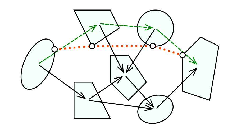
SPP in Graphs of Basic Semi-Algebraic Sets
Given the SPP in GBSAS:
I have not yet written up this step precisely, so this is a bit hand-wavy
-
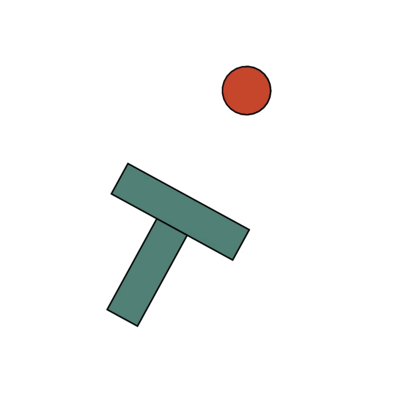
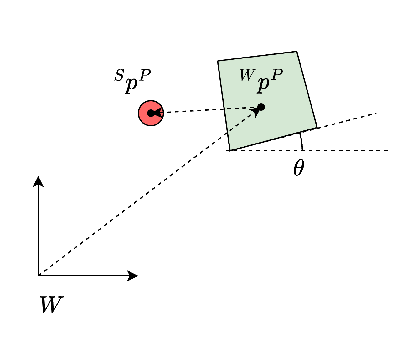
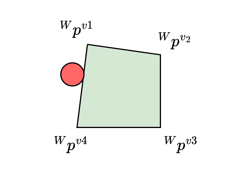
Let \( W\) denote the inertial frame
-
Let the slider be a polygon with \(N_F\) faces
-
Define \( ({}^W p^S, \theta) \in SE(2) \) as the pose of slider
-
-
The pusher is defined as a circle with radius \( R \in \R\)
-
Define \( {}^S p^P \in \R^2\) as the position of the pusher (in the \(S\) frame)
-
-
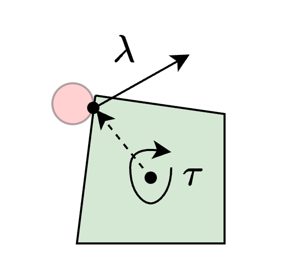
Define \( \lambda \in \R^2 \) as the contact force applied by the pusher on the slider (in the \(S\) frame)
Motion Planning for Planar Pushing (1/8)
-
We will assume quasi-static dynamics:
-
Assume no work done by impacts
-
Assume inertial forces are negligible
-
-
Work with dimensionless time
-
Assume isotropic friction
Motion Planning for Planar Pushing (2/8)
Motion Planning for Planar Pushing (3/8)
-
For \( m \in \mathcal{M} \), represent the motion with trajectory segment \[\xi_m = ((x_0, u_0), \ldots, (x_{N_m}, u_{N_m})) \in (\R^{N_x+N_u})^{N_m}\]
-
Where \( x_k = ({}^W p^S_k, \ c_{\theta,k}, \ s_{\theta,k}, \ {}^S p^P_k)\) and \( u_k = (\lambda_k, \Delta {}^S p^P_k) \)
-
\( c_\theta\) and \( s_\theta \) represent \( \cos(\theta)\) and \(\sin(\theta)\)
-
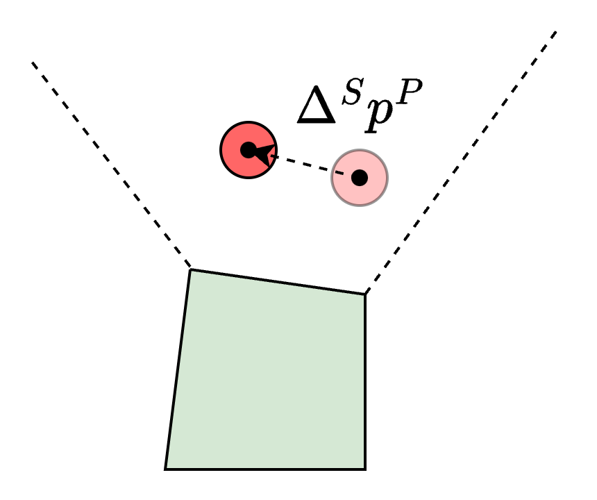
\(\Delta p_k = p_{k+1} - p_{k}\) denotes the displacement at knot point \(k\)
-
We consider two types of contact modes:
- Face-contact: Sticking contact between the slider and pusher at a face of the polytope (slider is sliding on table)
- Non-collision: Non-collision between pusher and slider (slider is sticking on table)
Motion Planning for Planar Pushing (4/8)
Non-collision
Face-contact
-
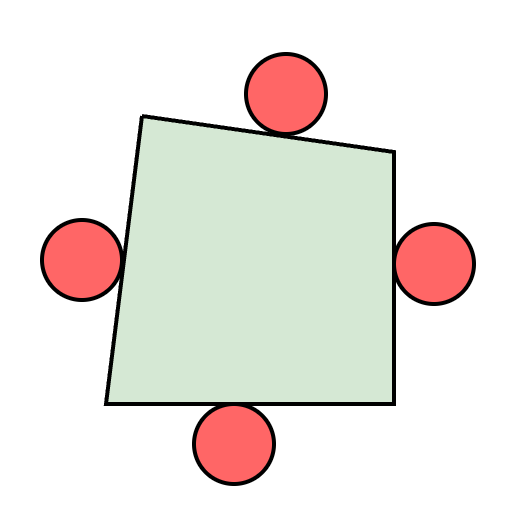
Associate a face-contact mode \(f_i \) with each face \(i = 1, \ldots, N_F\) of the slider
-
We are given a set \( \set{\mathcal{R}_1, \ldots, \mathcal{R}_{N_R} }\) of \(N_R\) collision-free regions for \( {}^S p^P \) (in the \(S\) frame)
Motion Planning for Planar Pushing (5/8)
\(f_1\)
\(f_2\)
\(f_3\)
\(f_4\)
Face-contact modes:
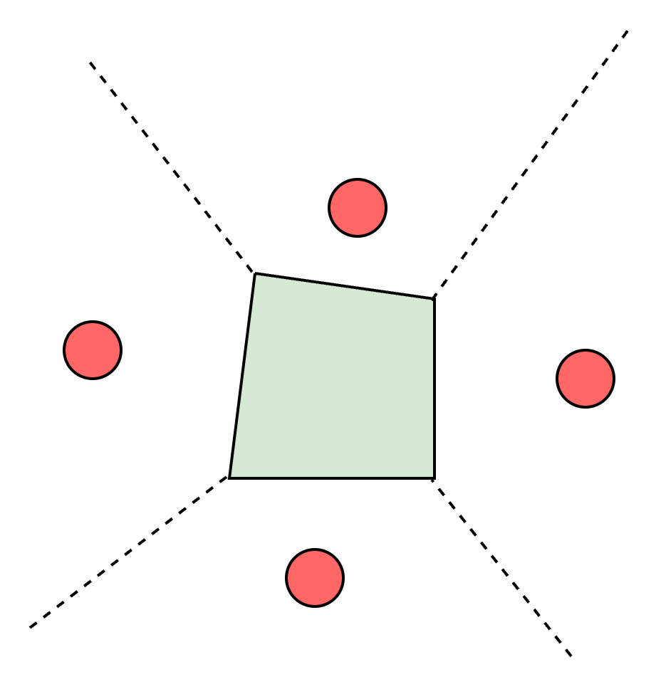
\(\mathcal{R}_1\)
\(\mathcal{R}_2\)
\(\mathcal{R}_3\)
\(\mathcal{R}_4\)
Collision-free regions:
Motion Planning for Planar Pushing (6/8)
-
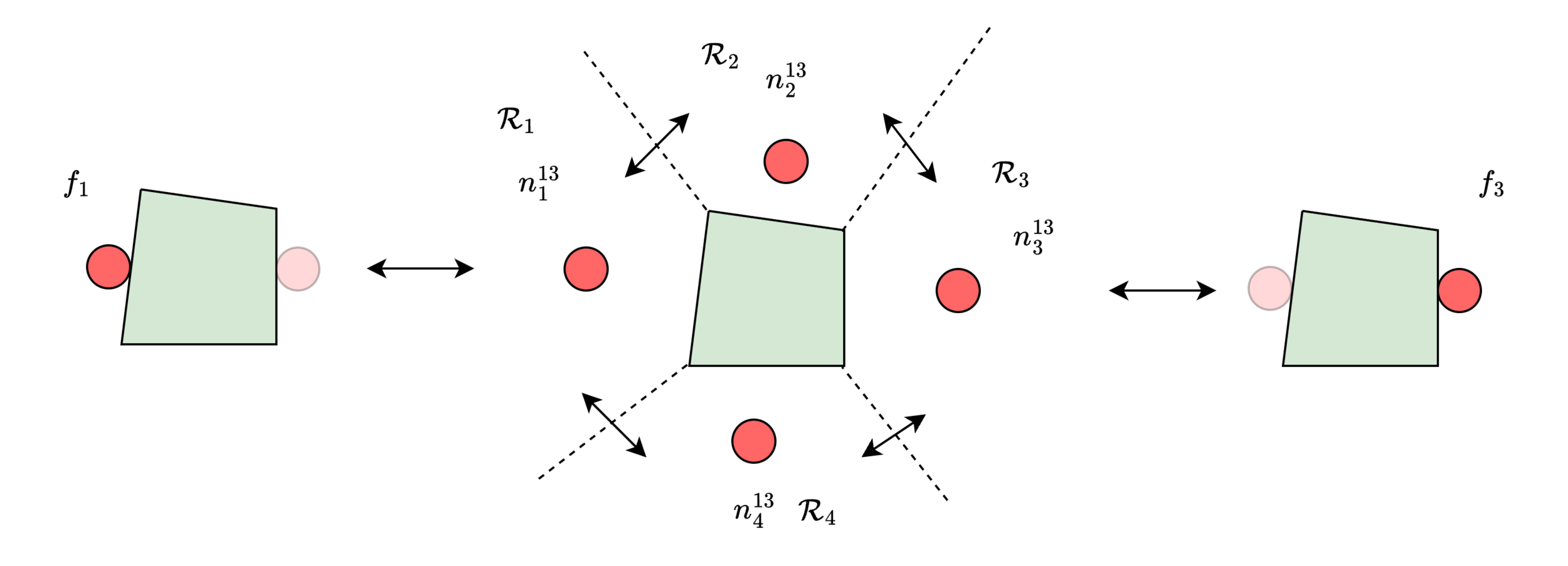
For each pair \((f_i, \, f_j), \, i \neq j \), we associate \(N_R\) non-collision modes \(n^{ij}_{1}, \ldots, n^{ij}_{N_R}\)
-
Let \(\mathcal{F} = \set{f_1, \ldots, f_{N_F}}\)
-
Let \(\mathcal{N} = \bigcup_{i \neq j} \set{n^{ij}_1, \ldots, n^{ij}_{N_R}}\), where \(i = 1,\ldots,N_F, \, j = 1, \ldots, N_F\)
-
Let \(\mathcal{M} = \mathcal{F}\cup\mathcal{N}\) be the set of all contact modes
-
We then have \(|\mathcal{M}| = N_F + N_R \binom{N_F}{2}\)
-
For \(i = 1,\ldots,N_F, \, j = 1, \ldots, N_F, \, i \neq j\):
-
Let \(\mathcal{T^{ij}_N}\) be the set of all bi-directional transitions \( (n^{ij}_k, n^{ij}_l) \) where \(\mathcal{R}_k \cap \mathcal{R}_l \neq \emptyset\)
-
Transitions between non-collision modes
-
-
Let \(\mathcal{T^{ij}_F},\) be the set of bi-directional transitions \( (f_i, n^{ij}_i )\) and \((n^{ij}_j,f_j) \)
-
Transitions between non-collision and face-contact modes
-
-
-
Let \(\mathcal{T} = (\bigcup_{i \neq j} \mathcal{T}^{ij}_N)\cup(\bigcup_{i \neq j} \mathcal{T}^{ij}_F)\)
Motion Planning for Planar Pushing (7/8)
-
We have now defined \(\mathcal{M}\), \(\mathcal{T}\), and \( \xi_m, \, m \in \mathcal{M}\)
-
We can (almost) solve the problem as a SPP in a graph of basic semi-algebraic sets:
-
We just need to define cost, dynamics, state and input constraints for all modes \( m \in \mathcal{M} \)
Motion Planning for Planar Pushing (8/8)
- Let \( f \in \mathcal{F} \) be a face-contact mode
- Let \( {}^W p ^{v_i} = {}^W p ^{v_i}(x), \, i = 1, \ldots, N_V \) denote the position of vertex \(i\) of the slider in \(W\)
- Note that \( {}^W p ^{v_i} \) is a linear function of \( x \)
- Define the mode cost as \[ l_f(\xi_f) = \sum_{k=1}^{N_f - 1} \left( \frac{1}{N_V} \sum_{i=1}^{N_V} \|\Delta {}^W p^{v_i}_k \|^2 + \| \lambda_k \|^2 \right) + C\]
- Where \( C \in \R\) is a constant
- We minimize squared displacements on fixed keypoints on slider, as well as squared contact forces
Face-Contact Modes (1/6)
The limit surface (1/2)
- Let \(\tau = \tau(x,u) \in \R\) be the induced contact torque (a quadratic function in \(x\) and \(u \))
- Let the limit surface be defined by: \[ \set{y = (\lambda, \tau) \mid H(y) = 0 } \subset \R^3, \, H: \R^3 \rightarrow \R \]
- Use an ellipsoidal approximation of the limit surface: \[ H(y) = \frac{1}{2} y^\intercal D y - 1, \, D = \text{diag}((c_\lambda, c_\lambda, c_\tau))\]
- Where \( c_\lambda, \, c_\tau \) are constants depending on the geometry of the slider
Face-Contact Modes (2/6)
The limit surface (2/2)
- Sliding between slider and table: \((\lambda, \tau)\) must lie on the limit surface, and the slider displacement perpendicular to the surface: \[ (\Delta {}^W p^S, \Delta \theta) \propto \nabla H((\lambda, \tau)) = \frac{1}{2} D\begin{bmatrix}\lambda \\ \tau\end{bmatrix}\]
- Gradient of the limit surface is \(\nabla H(y) = (1/2) Dy\)
- Trick: We have non-dimensional time, so we enforce \[ \begin{bmatrix}\Delta {}^W p^S\\ \Delta \theta\end{bmatrix} = \frac{1}{2} D\begin{bmatrix}\lambda \\ \tau\end{bmatrix}\] and scale \((\lambda, \tau)\) as a post-processing step
Face-Contact Modes (3/6)
- The dynamics for the mode \( f \) are then given by:
- Where \( \begin{bmatrix}\Delta {}^W p^S_k\\ \Delta \theta_k\end{bmatrix} = \frac{1}{2} D\begin{bmatrix}\lambda_k \\ \tau_k(x)\end{bmatrix}\)
- These are quadratic in our choice of state and input
- (The last equation is implicit, arising from the relationship between \(SO(2)\) and \(\mathfrak{so}(2)\), assuming \(\Delta \theta \approx 0 \). Think of \(\Omega = \dot R R^T\))
Face-Contact Modes (4/6)
- Let the input constraint polytope \(\mathcal{U}_f\) be defined by
- where \(\lambda_n\) and \(\lambda_f\) are the normal and frictional components of \(\lambda\), and \(\mu\) is the friction coefficient between the pusher and slider
- I.e. we enforce sticking between slider and pusher, and friction cone constraints
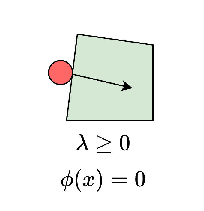
Face-Contact Modes (5/6)
Face-Contact Modes (6/6)
- Let the state constraint set \(\mathcal{X}_f\) be defined by
- Where \( \phi \) is the signed-distance function (linear in our choice of state)
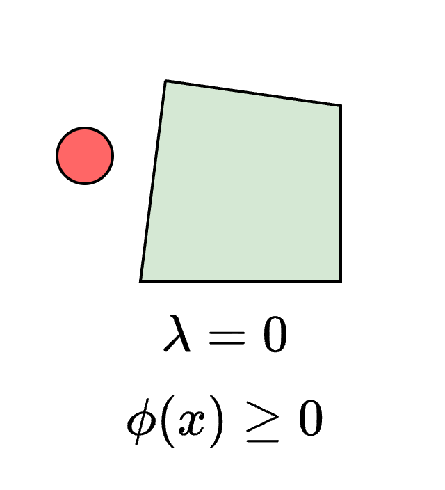
Non-Collision Modes (1/2)
- Let \( n \in \mathcal{N} \) be a non-collision mode
- Then we define the dynamics \( f_n \) such that:
- I.e. slider stays still, and we directly command position of the pusher
- We define the input constraint polytope \(\mathcal{U}_n\) by \( \lambda_{k} = 0, \, k = 1, \ldots, N_n - 1\)
- Let \(\mathcal{R}\) be the collision-free region associated with \(n\)
- We define the state constraints set \(\mathcal{X}_n\) by \( {}^S p^P_k \in \mathcal{R}, \, k = 1, \ldots, N_n - 1 \)
- Also a polytope in this case
- We define the cost \( l_n \) by \[l_n(\xi_n) = \sum_{k=1}^{N_n-1} \| \Delta {}^S p_k^P \|^2 + \sum_{k=2}^{N_n-1} \frac{1}{\phi_m({}^S p^P_k)} \]
- Minimize squared Euclidean displacements
- Maximize distance to object
Non-Collision Modes (2/2)
Method summary
- Given the slider geometry, pusher radius, start configuration and end configuration we solve:
- (or the "semidefinite relaxation" of this)
Results - Motion Plans
- Generated in ~6 seconds
- Generated in ~6 seconds
- Generated in ~1 minute
Results - Simulated "real" system
- We simulate the plans in Drake on a Kuka Iiwa with a "finger"
- Use hydroelastic contact simulation
- Use hybrid MPC controller with "family of modes" as in [2]

- Shao has been helping with implementing the Hybrid MPC controller (thank you Shao)!
[2] F. R. Hogan, E. R. Grau, and A. Rodriguez, “Reactive Planar Manipulation with Convex Hybrid MPC,” in 2018 IEEE International Conference on Robotics and Automation (ICRA), May 2018
Results - Simulated "real" system
Open loop
Closed loop
Results - Simulated "real" system
Open loop
Closed loop
Discussion
- Given a slider with \( N_F \) faces
- In theory complexity should scale roughly with \( O(N_F^2 )\) (from \( \binom{N_F}{2} \) edges between contact modes )
- (If we are ignoring non-collision modes)
- It seems we are seeing worse than this in practice
- Reason is a bit unclear, could be numerics or something I haven't yet thought about
Complexity
Discussion
- How to evaluate tightness?
- Look at violation of quadratic equality constraints
- For rotations in \( (-\pi/2, \pi/2) \) we seem to often be getting good solutions
- In-place rotation gives looser solutions
- For higher rotations we are getting loose solutions
- Unclear if caused by GCS or SDP relaxation (or both), will need to look more into this!
Tightness
Future work
- Obstacle avoidance
- In-plane manipulation
- Decomposition algorithms to speed things up?