Motion Planning for
Planar Pushing using GCS
Robot Locomotion Group, MIT
Short Talk, Spring 2023
Bernhard Paus Græsdal
Problem Formulation
Problem definition
Decision variables
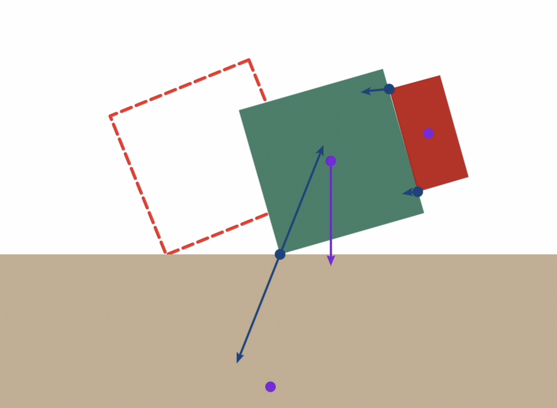
- Object pose: \( {}^W p^B \in \mathbb{R}^2, {}^W R^{B} \in SO(2) \)
- Finger position \( {}^B p^F \in \mathbb{R}^2\)
- Contact force \( f^F_B \in \mathbb{R}^2 \)
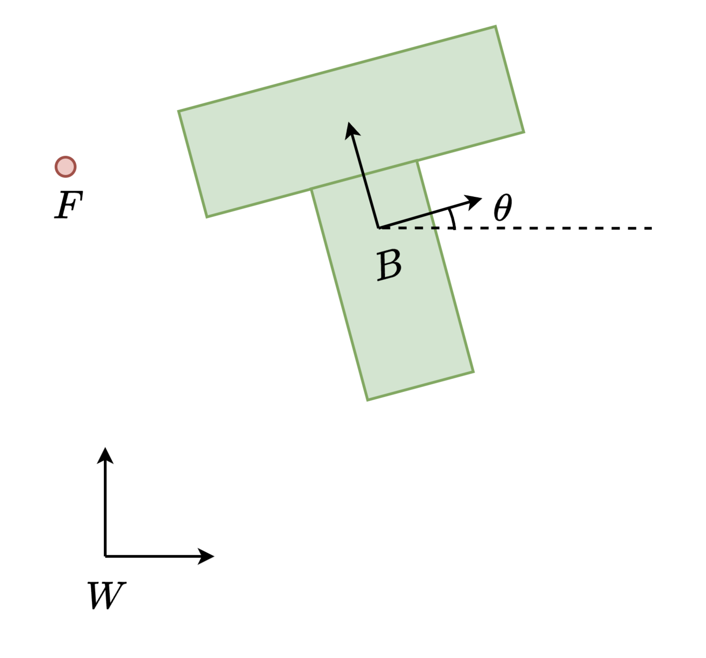
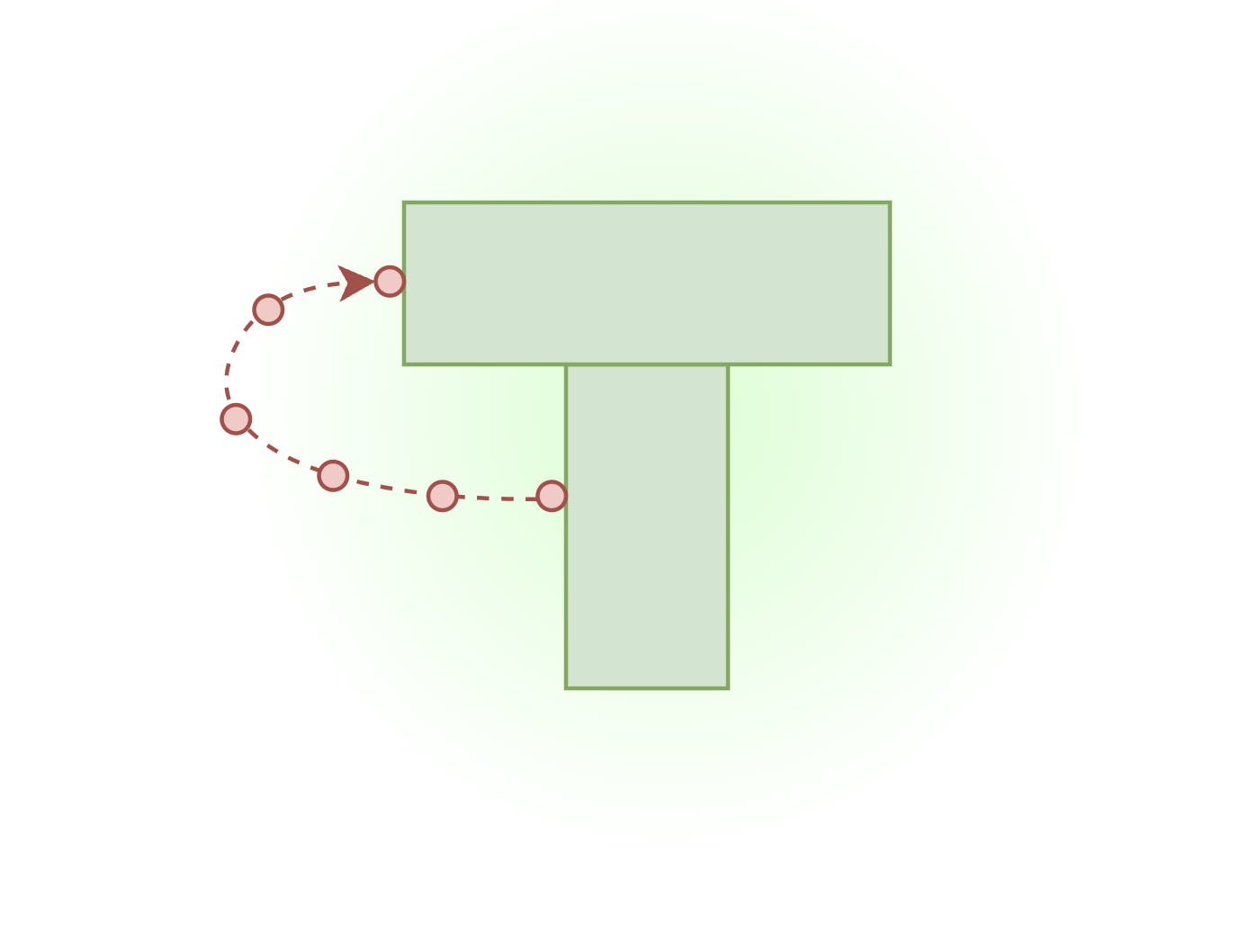
- Task: Given initial and final pose for T-object, find the optimal trajectory
- \( \implies \) Formulate this as a GCS problem!
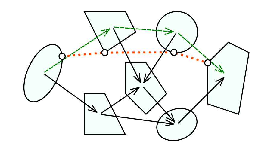
Graph-of-Convex-Sets
- Directed graph \( G = (\mathcal{V}, \mathcal{E}) \)
- Bounded convex sets \( \mathcal{X}_v \)
- Source and target \( \sigma, \tau \in \mathcal{V} \)
- \( \mathcal{P} \) family of all \( \sigma-\tau \) paths in \( G \)
- \( \mathcal{E}_p \) set of edges traversed by path \( p \in P \)
- Convex edge lengths \( l_e(x_u, x_v) \geq 0 \)
- Convex edge constraints \( \mathcal{X}_e \)
[1] T. Marcucci, J. Umenberger, P. A. Parrilo, and R. Tedrake, “Shortest Paths in Graphs of Convex Sets.” 2022.
[2] T. Marcucci, M. Petersen, D. von Wrangel, and R. Tedrake, “Motion Planning around Obstacles with Convex Optimization.” 2022.
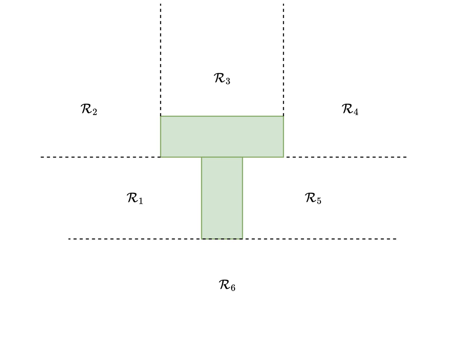
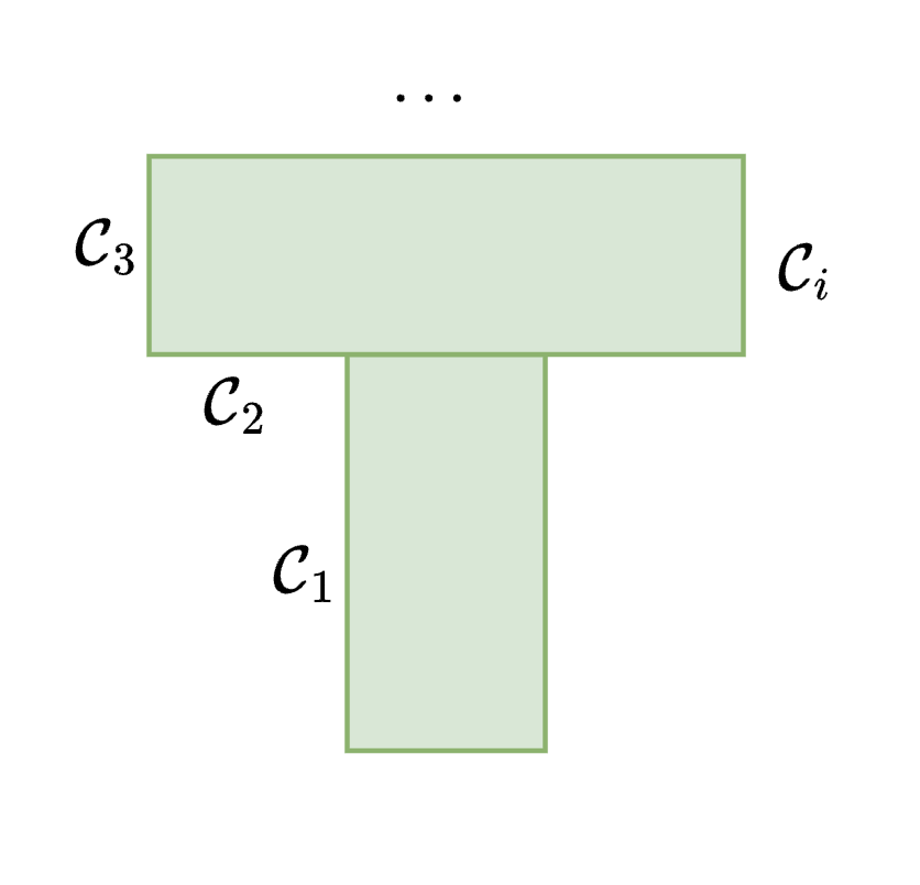
The Graph for Planar Pushing
Two types of vertex sets \( \mathcal{X}_v \)
- \( \mathcal{R}_j \) Collision-free sets for collision-free region \(j\)
\( \rightarrow \) Polytope - \( \mathcal{C}_i \) sticking contact to face \(i\)
\( \rightarrow \) Spectrahedron (after SDP relaxation)
The Vertices / Convex sets
The Vertices
1. Non-collision modes \( \mathcal{R}_j \)
- \( N_{\mathcal{R}} \) knot points
- Decision variables:
\( {}^B p^F_k, \, k = 1,\ldots,N\)
\( {}^W p^B_l, {}^W R^{B}_l, \, l \in \left \{ 1, N \right \} \) - Set defined by non-collision
\( \mathcal{X}_v = \left\{ {}^B p^F \lvert A ({}^B p^F_k) + b \geq 0, \forall k \right\} \) - Edge constraints \( \mathcal{X}_\mathcal{E} \) are continuity constraints on first and last knot point
[1] N. Chavan-Dafle, R. Holladay, and A. Rodriguez, “Planar in-hand manipulation via motion cones,” Mar. 2020
[2] F. R. Hogan, E. R. Grau, and A. Rodriguez, “Reactive Planar Manipulation with Convex Hybrid MPC,” 2018
- \( N_{\mathcal{C}} \) knot points
- Decision variables:
Object pose: \( {}^W p^B_k, {}^W R^{B}_k \)
Finger position \( {}^B p^F_k\)
Contact force \( [f^c_B]_k\)
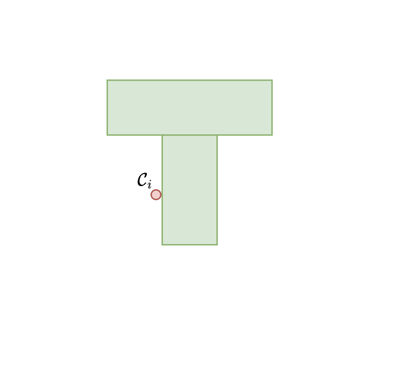
The Vertices
2. Contact with face \( \mathcal{C}_i \)
[1] N. Chavan-Dafle, R. Holladay, and A. Rodriguez, “Planar in-hand manipulation via motion cones,” Mar. 2020
[2] F. R. Hogan, E. R. Grau, and A. Rodriguez, “Reactive Planar Manipulation with Convex Hybrid MPC,” 2018
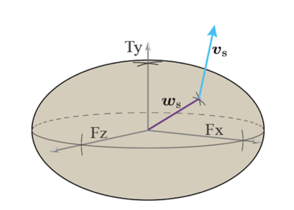
- Using an ellipsoidal limit surface approximation and quasi-static dynamics we obtain
The Vertices
\( \leftarrow \) Quadratic (non-convex) in \( x_k, u_k \)
- Ellipsoidal approximation: During sliding, friction wrench intersects limit surface, and object twist must be perpendicular to limit surface
\( t_B = Aw_B, \quad A = \text{diag}([\frac{1}{f_{max}^2}, \, \frac{1}{f_{max}^2}, \, \frac{1}{\tau_{max}^2}]), \quad \frac{1}{2} w^\intercal A w = 1 \)
2. Contact with face \( \mathcal{C}_i \)
The Vertices in GCS
2. Contact with face \( \mathcal{F}_i \)
\( \longrightarrow \)
\( X := xx^\intercal \)
- Turn (quadratic) basic semi-algebraic set into a spectrahedron using SDP relaxation:
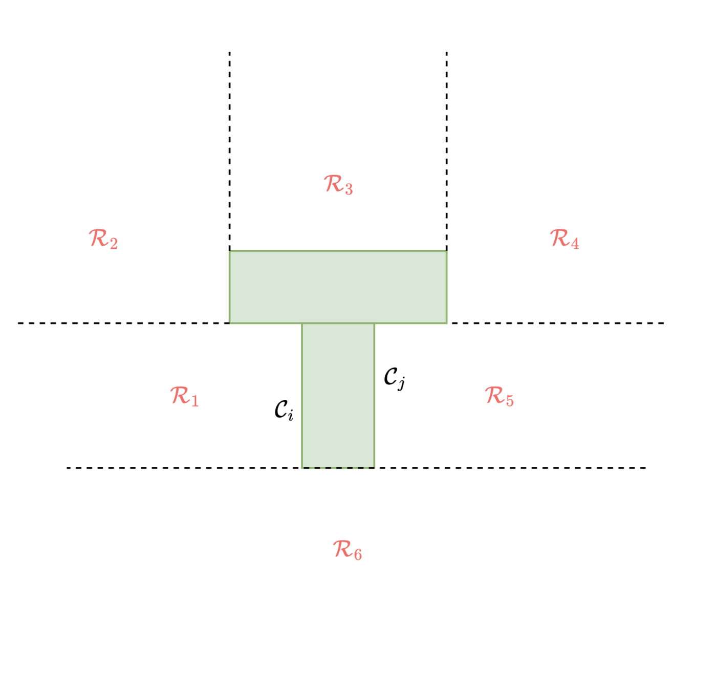
Edge Connections
- Transition from any contact mode to any contact mode
- ... While staying collision free
Edge Connections
- Non-collision subgraph of polytopes \( \mathcal{R}_i \) between every two pairwise spectrahedrons \( \mathcal{C}_i, \mathcal{C}_j \)
- Edge constraints \( \mathcal{X}_\mathcal{E} \)
- Continuity on object pose \( {}^W p^B, {}^W R^B \)
- Continuity on finger position \( {}^B p^F \)
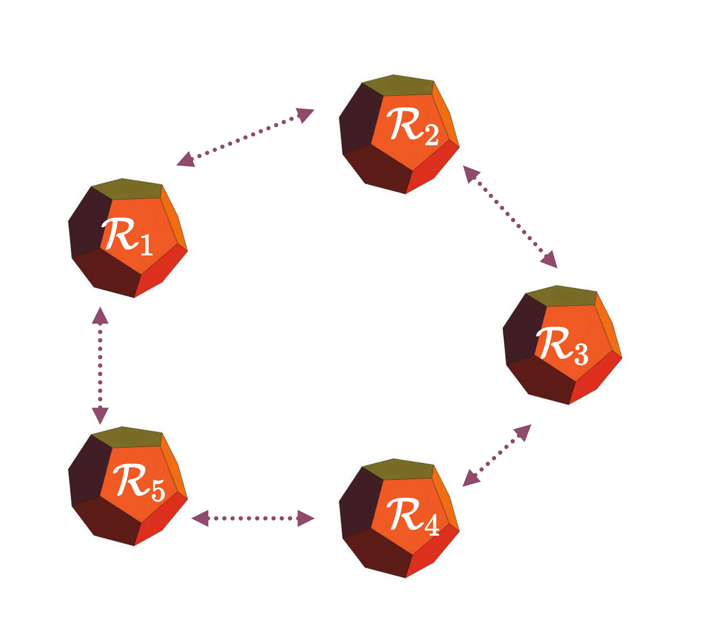
The Graph for Planar Pushing
Final graph
- Contact modes connected through subgraphs
- Source and target nodes are singletons
- Connected to every contact mode
- Continuity on object pose \( {}^W p^B, {}^W R^B \)
Vertex costs
Contact modes \( \mathcal{C}_i\)
Non-collision \(\mathcal{R}_j\)
- Minimize kinetic energy
- SDP relaxation for \(SO(2)\) is tight
(gives a linear cost term in original variables)
- Minimize Euclidean distance
[1] N. Chavan-Dafle, R. Holladay, and A. Rodriguez, “Planar in-hand manipulation via motion cones,” Mar. 2020
\( f_{max}, \tau_{max} \) = Maximum frictional force/torque from table
- Using an ellipsoidal limit surface approximation and quasi-static dynamics:
The Vertices in GCS
2. Contact with face \( \mathcal{C}_i \)
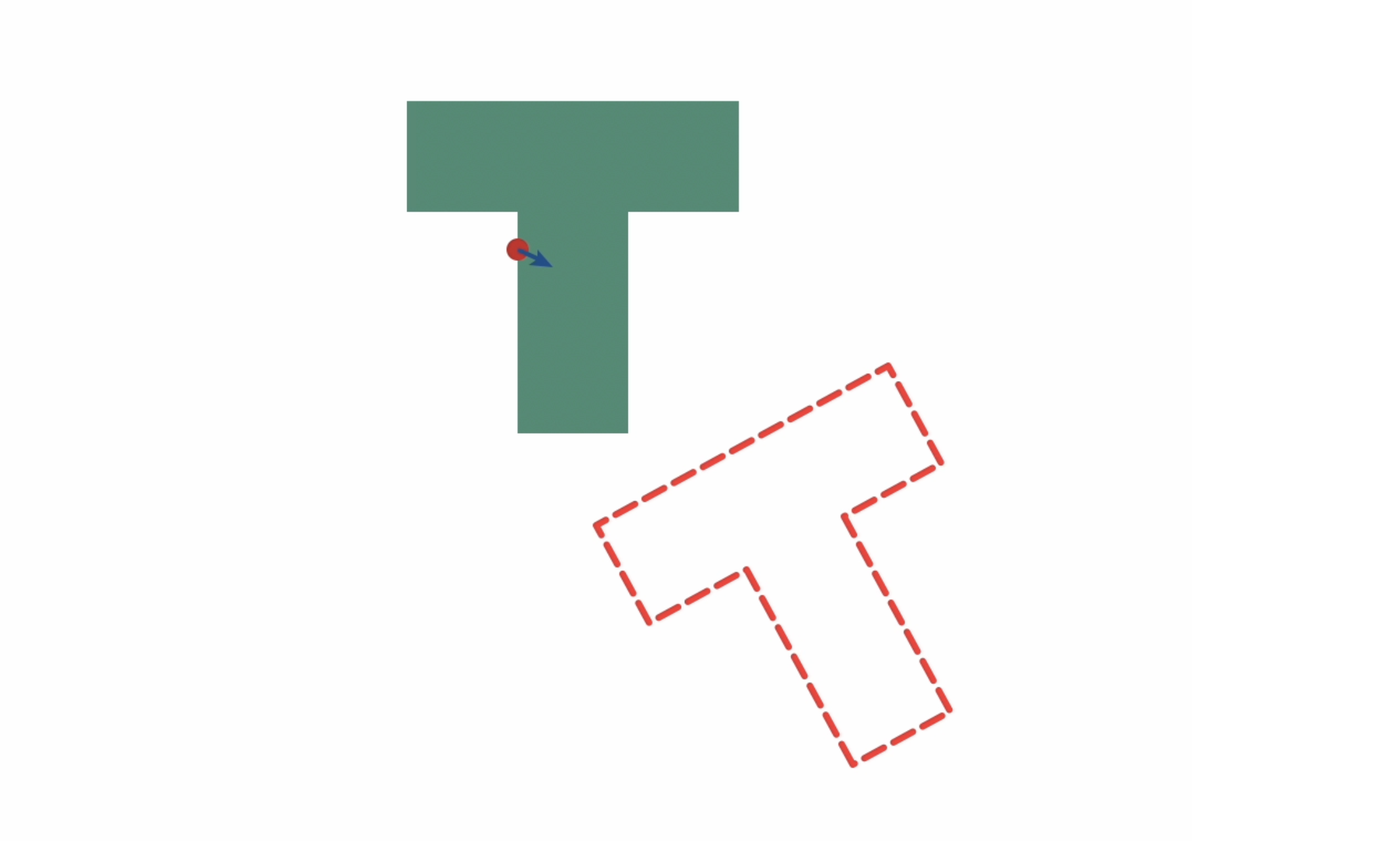
Preliminary Results
Pushing for the T-object
Future directions
Moving away from the object
- Now we are only using 2 knot points for collision-free sets \( \mathcal{R}_j \)
- Let SDF be \( \phi(x) \)
-
Ideally we want a log barrier cost:
\( \min_x -\log{\phi(x)} \)
Other directions
- Evaluate relaxation error
- Test trajectories in Drake
- Replace contact model
(use point contacts at vertices of convex hull of object)
\( \implies \) More accurate model
Other directions
- Extend object manipulation with planning over modes using GCS: