Planning Through Contact with Trajectory Optimization and GCS

Robot Locomotion Group, MIT

Long Talk, Spring 2023

Bernhard Paus Græsdal

Why do we care about planning through contact?

Current systems are task-specific
We want a general planning framework for novel manipulation tasks
Combinatorial blowup and non-convexity makes motion planning a big challenge

Relevant Work

How is the problem solved today?

Typical tools of choice

1. Sampling-Based Planning

2. Trajectory Optimization

Russ Tedrake. Underactuated Robotics: Algorithms for Walking, Running, Swimming, Flying, and Manipulation (Course Notes for MIT 6.832)

Figures borrowed from:

1. Sampling-Based Manipulation Planning

Advantages

Takes robot kinematics into account
Doesn't explicitly reason about contact modes

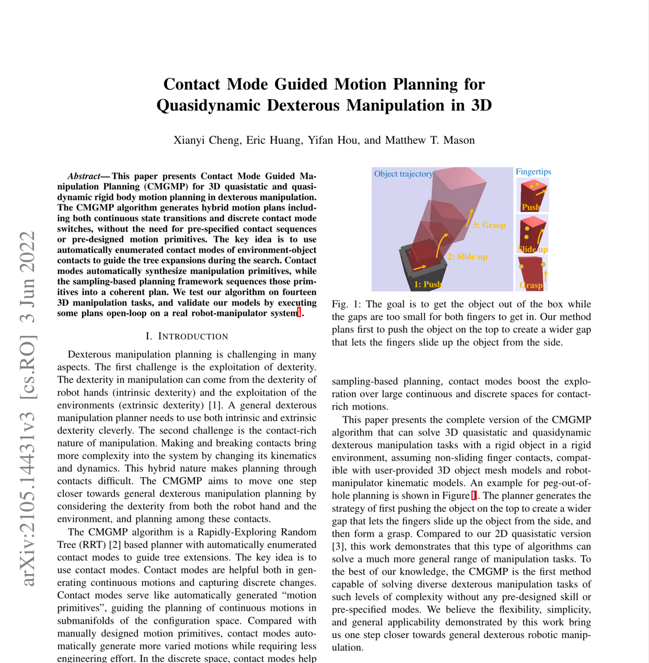
Mode Sampling and projection onto contact manifold + RRT

Smooth dynamics + Reachability metric + RRT

Drawbacks

Suffers the curse of dimensionality
The "RRT"-dance

2. Contact-Rich Trajectory Optimization

Nonlinear optimization + Implicit contact modes (complimentarity condition)

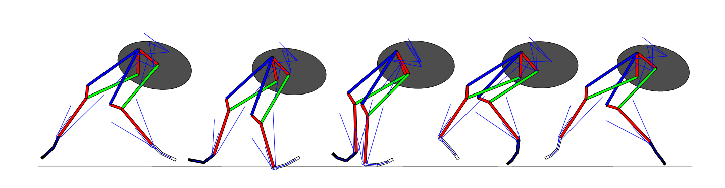
Mixed-Integer Convex Problem + Pre-specified trajectories + McCormick Relaxations

Advantages

Works well with pre-defined mode schedules
(used a lot for locomotion)
(Local) optimality

Disadvantages

Very hard when you also search over contact modes
Non-convex in the general case with rotations
For non-convex trajopt: reliant on initial guess and tuning

Sampling-Based Manipulation Planning

Takes robot kinematics into account
Doesn't explicitly reason about contact modes
Suffers the curse of dimensionality

Smooth dynamics + Reachability metric + RRT

Sampling-Based Manipulation Planning

Mode Sampling and projection onto contact manifold + RRT

TODO

Contact-Rich Trajectory Optimization

Nonlinear optimization + Implicit contact modes (complimentarity condition)

Non-convex
??
??

Contact-Rich Trajectory Optimization

Works well with pre-defined mode schedules
(used a lot for locomotion)
Hard when you search over contact modes

Nonlinear optimization + Implicit contact modes (complimentarity condition)

Contact-Rich Trajectory Optimization

Mixed-Integer Convex Problem + McCormick Relaxations

Exponential in the number of contact modes
Scales poorly
TODO add videos?

Our Approach

Plan Through Contact Modes using GCS

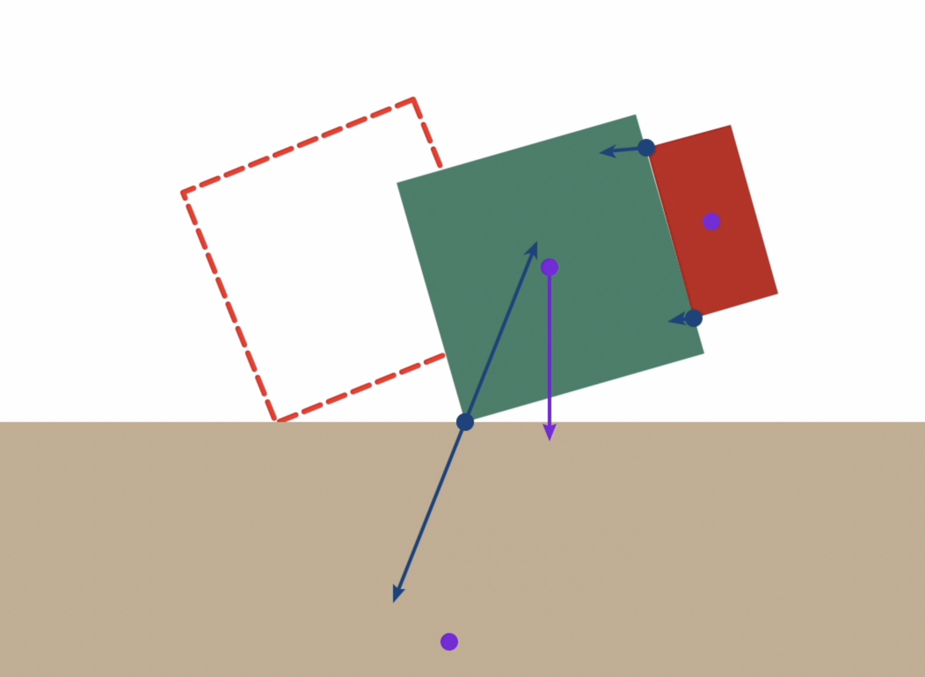
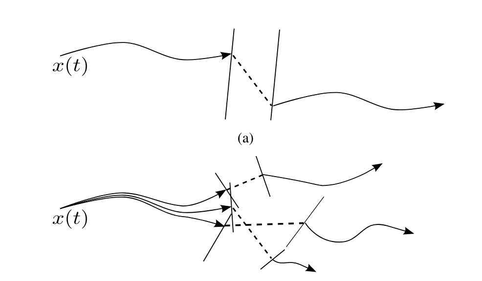
How to flip up and push the object?

To plan this motion, we need to simultaneously decide:

Contact mode sequence
Continuous motion within each contact mode

Motivational Example

[1] N. Doshi, O. Taylor, and A. Rodriguez, “Manipulation of unknown objects via contact configuration regulation.” arXiv, Jun. 01, 2022. doi: 10.48550/arXiv.2203.01203.

Figure taken from [1]

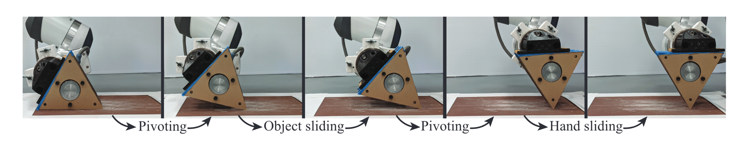
The task at hand

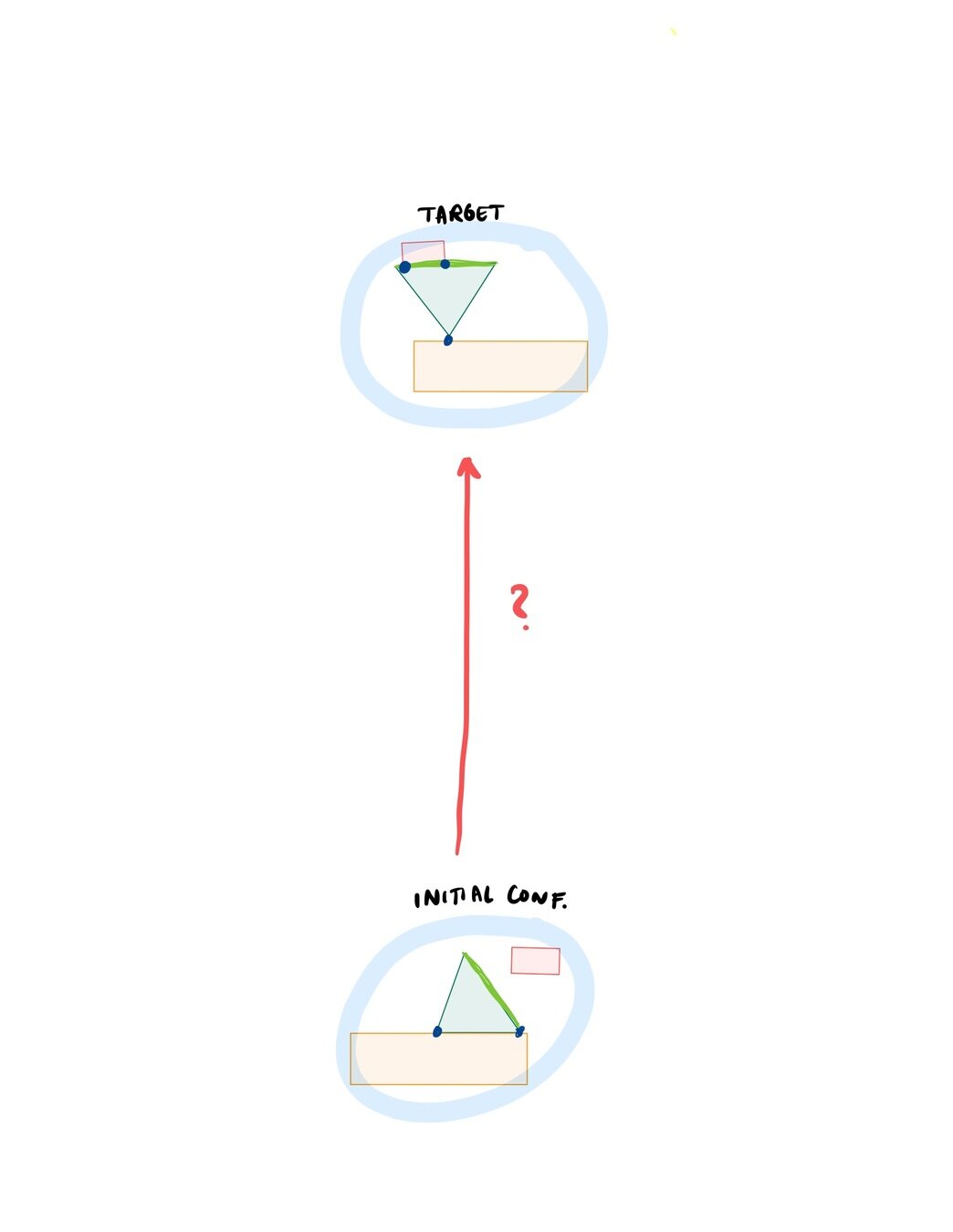
We want to...

Flip up the object
Push the object
Reposition the end-effector

... in no particular order

While minimizing some quantity:

Kinetic energy
Exerted work
...

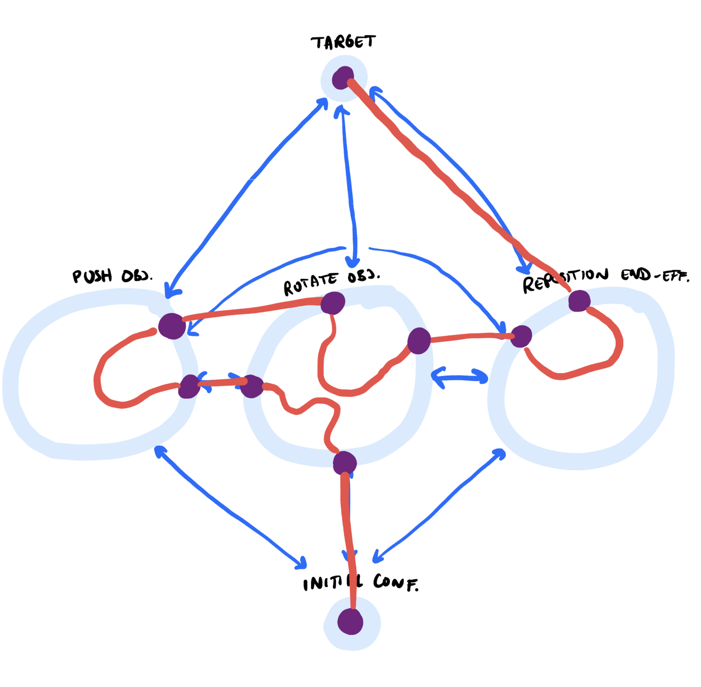
Let's build a graph

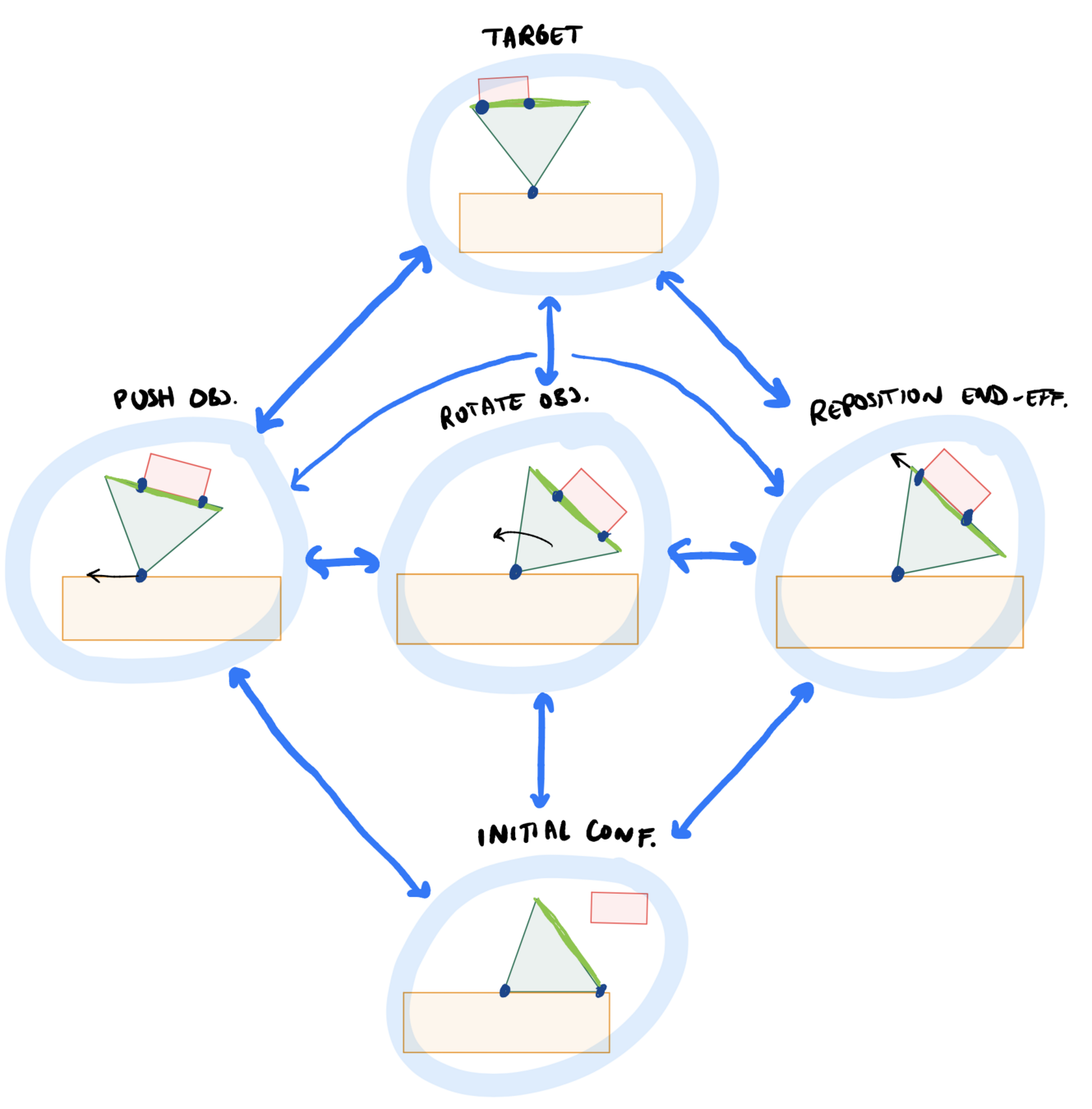
Each contact mode is a set!
Initial and target configurations are singletons

Let's build a graph

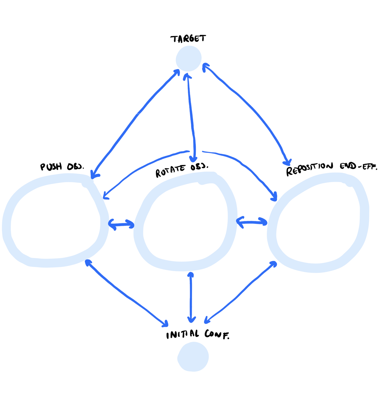
More abstractly, we get a graph like this:

Let's build a graph

If we can solve the SPP, we have our plan!

\Updownarrow

Our Approach

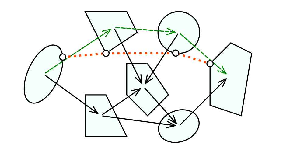
Plan through contact using GCS

\implies

Sets are contact modes

There's a problem with this picture...

Can we plan through contact modes with GCS?

Generally, no!

Contact modes are non-convex
However, the sets are basic semi-algebraic!

We need to find a convex formulation (relaxation) for the contact modes

Preliminary Results

Planning within one contact mode

Object Flip-Ups & Pushing

Object Flip-Ups

Planar Pushing

Planning Through Contact Modes with GCS

(In the convex, non-rotational case)

Problem Formulation

Making the contact modes convex

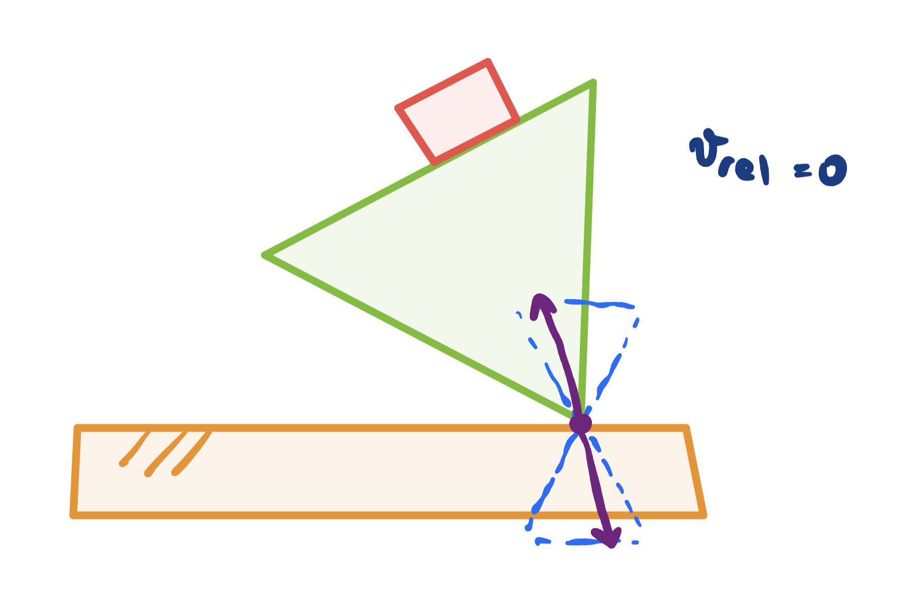
Contact Modelling

Modelling Choices

Modelling decisions (1/2):

Assume quasi-static dynamics:
- Low velocities, low inertial forces and no impacts
(Quasi-dynamic: Allows brief periods of dynamic motion, but assumes accelerations do not integrate into significant velocities)

\begin{aligned} M (q) \dot{{v}} + {C} (q, v) v = &\tau_g(q) + \sum_i J_{c,i}^\intercal f^{c_i} \\ M (q) \dot{{v}} + {C} (q, v) v \approx 0 \implies &\tau_g(q) + \sum_i J_{c,i}^\intercal f^{c_i} = 0 \end{aligned}

Modelling Choices

Modelling decisions (2/2)

Use relative quantities in frames of objects in contact
Minimize kinetic energy

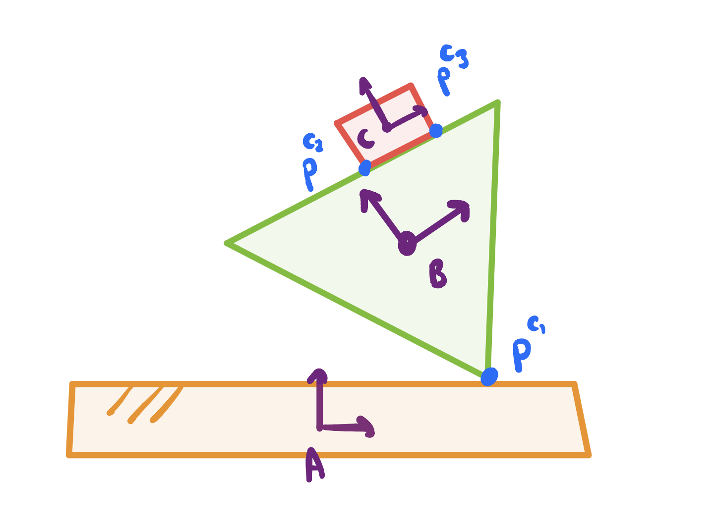
Defining Decision Variables

Relative positions
Relative rotation
Contact positions (in local frames)
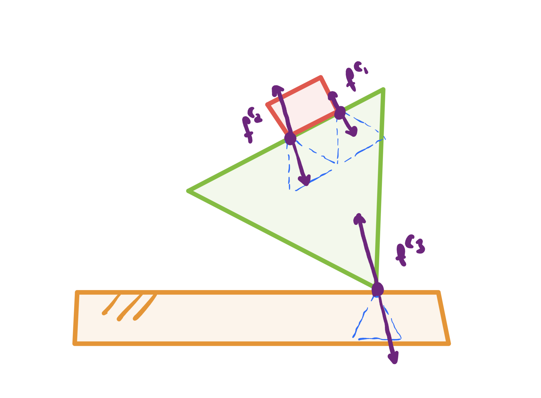
Contact forces

{}^A p^B, {}^B p^A \in \mathbb{R}^2

{}^A R^B \in SO(2)

(A,B)

For each active contact pair

{}p^{c_i}_A, \, {}p^{c_i}_B \in \mathbb{R}^2 \quad \\

f^{c_i}_A, f^{c_i}_B \in \mathbb{R}^2 \\ \quad \quad \forall i \in \text{Contact points}

For each knot point $ k = 0, \ldots , N $

Consistency across frames

Contact points equal
Relative positions consistent
Newton's third law for contact forces

where $W$ is some common frame

[{}^{{A}} p^{c_i}]_{{W}} = [{}^{{B}} p^{c_i}]_{{W}}

(A,B)

For each active contact pair

[{}^{{A}} p^{B}]_{{W}} = - [{}^{{B}} p^{A}]_{{W}}

[ {f}^{c_i}_{{A}} ]_{{W}} = -[ {f}^{c_i}_{{B}} ]_{{W}}.

Contact modes

\begin{aligned} c^{n_i} &\geq 0 \\ \left| c^{f_i} \right| &\leq \mu c^{n_i} \\ v_{\text{rel}} &= 0 \end{aligned}

Sticking contact

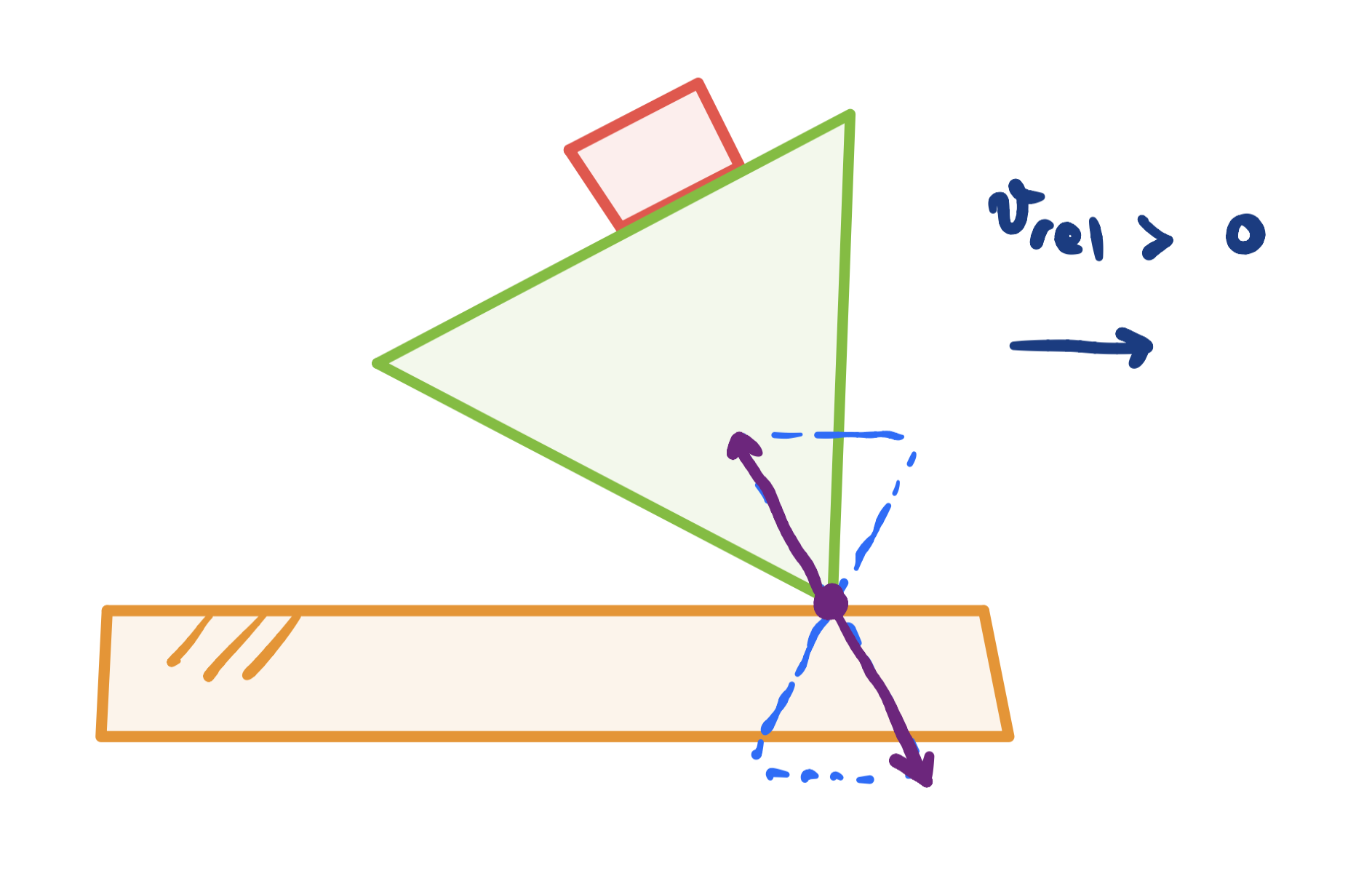
\begin{aligned} c^{n_i} &\geq 0 \\ \left| c^{f_i} \right| &= \mu c^{n_i} \\ v_{\text{rel}} &\geq 0 \quad \text{or} \quad v_{\text{rel}} \leq 0 \end{aligned}

2. Sliding contact

All constraints

\begin{aligned} \quad \tau_g(q) + \sum_i J_{c,i}^\intercal f^{c_i} &= 0 \\ \quad {}^A R^B &\in SO(2), \\ \quad f^{c_i} &\in \mathcal{FC}_i \\ \quad p^{c_i} &\in \text{Face} \, \text{or} \, \text{Vertex} \\ M R &\geq 0 \quad (\text{non-penetration}) \\ \quad [{}^{{A}} p^{c_i}]_{{W}} &= [{}^{{B}} p^{c_i}]_{{W}} \\ \quad [{}^{{A}} p^{B}]_{{W}} &= - [{}^{{B}} p^{A}]_{{W}} \\ \quad [ {f}^{c_i}_{{A}} ]_{{W}} &= -[ {f}^{c_i}_{{B}} ]_{{W}} \\ \quad \forall (A,B) &\in \text{Contact Pairs} \\ \quad \forall i &\in \text{Contact Points} \end{aligned}

(for planning within one contact mode)

Non-convex

(quadratic equality constraints)

(knot point indices omitted for notational simplicity)

Cost

We assume low velocities
$ \implies $ Minimize kinetic energy over the trajectory

\begin{aligned} K &= \int_0^T \left[ \frac{1}{2}m \lVert v (t) \rVert^2 + \frac{1}{2} I \lVert \omega (t) \rVert ^2 \right] dt \end{aligned}

$ v(t) = \dot p(t) $
In general $ [\omega]^\times = \dot R R ^ \intercal $. We obtain $ \lVert \omega \rVert ^2 $ as

\begin{aligned} \lVert \omega (t) \rVert ^2 = \omega ^\intercal \omega = \frac{1}{2} \text{vec}(\dot R)^\intercal \text{vec}(\dot R) &:= \frac{1}{2} \lVert \dot r(t) \rVert^2 \\ r &:= \text{vec}(R) \end{aligned}

(Proof on next slide)

\begin{aligned} \implies K &= \int_0^T \left[ \frac{1}{2}m \dot p(t)^\intercal \dot p(t) + \frac{1}{4} I \dot r(t)^\intercal \dot r(t) \right] dt \end{aligned}

Cost

(Proof):

\begin{aligned} \implies \lVert \omega \rVert ^2 = \omega ^\intercal \omega &= \frac{1}{2} \text{Tr}([\omega]^\times {}^\intercal [\omega]^\times) = \frac{1}{2}\text{Tr}(R \dot R^\intercal \dot R R^\intercal) \\ &= \frac{1}{2} \text{Tr}(\dot R^\intercal \dot R) = \frac{1}{2} \text{vec}(\dot R)^\intercal \text{vec}(\dot R) \\ &:= \frac{1}{2} \dot r^\intercal \dot r = \frac{1}{2} \lVert \dot r \rVert^2 \quad \quad \square \end{aligned}

\frac{1}{2} \text{Tr}([a]^\times {}^\intercal [a]^\times) = \text{vec}(a)^\intercal \text{vec}(a) = a^\intercal a

[\omega]^\times = \dot R R ^ \intercal

\text{Tr}(A^\intercal B) = \text{vec}(A)^\intercal \text{vec}(B)

Cost

\begin{aligned} K &= \int_0^T \left[ \frac{1}{2}m \dot p(t)^\intercal \dot p(t) + \frac{1}{4} I \dot r(t)^\intercal \dot r(t) \right] dt \end{aligned}

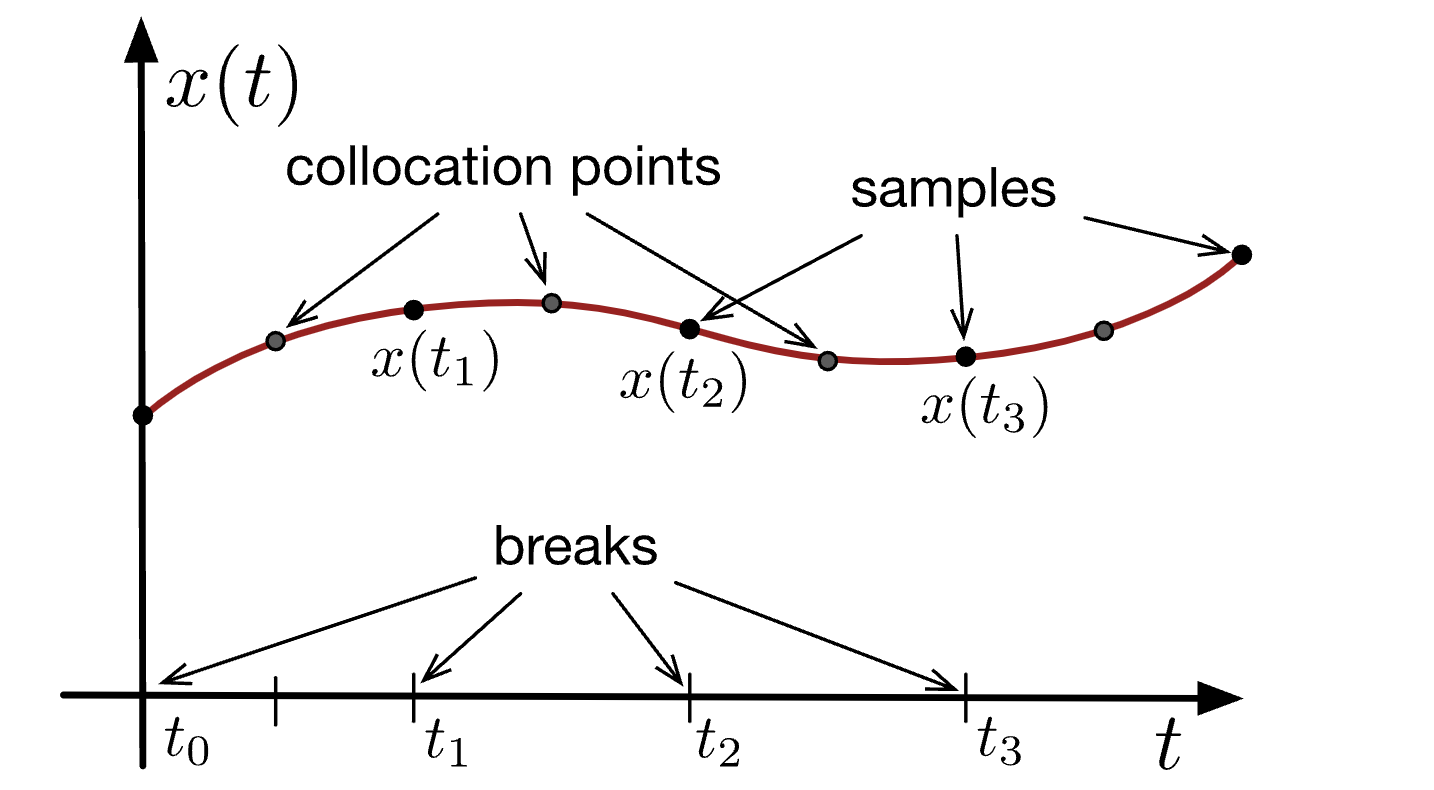
Use forward-differences to obtain derivatives

v[i] = \dot p[i] := \frac{1}{\Delta t} (p[i+1] - p[i])

Use Riemann-sums to approximate the integral
We thus minimize the following cost:

\begin{aligned} K &\approx \sum_{k=0}^{N} k_v (p_{k+1} - p_{k})^\intercal (p_{k+1} - p_{k}) + k_\omega (r_{k+1} - r_{k})^\intercal (r_{k+1} - r_{k}) \end{aligned}

Cost Summary

\begin{aligned} K &= \int_0^T \left[ \frac{1}{2}m \lVert v (t) \rVert ^2 + \frac{1}{2} I \lVert \omega(t) \rVert^2 \right] dt \\ &= \int_0^T \left[ \frac{1}{2}m \dot p(t)^\intercal \dot p(t) + \frac{1}{4} I \dot r(t)^\intercal \dot r(t) \right] dt \\ &\approx \sum_{k=0}^{N} k_v \lVert p_{k+1} - p_{k} \rVert^2 + k_\omega \lVert r_{k+1} - r_{k} \rVert^2 \end{aligned}

Minimizing kinetic energy of the trajectory

$ \Updownarrow $

Minimizing squared Euclidean distances directly in the coordinates of the position and rotation

Full Optimization Problem

\begin{aligned} \min_{p, p^{c_i}, f^{c_i}, R} \quad \sum_{k=0}^{N} k_v \lVert p_{k+1} - p_{k} \rVert^2 &+ k_\omega \lVert r_{k+1} - r_{k} \rVert^2 \\ \text{subject to} \quad \tau_g(q) + \sum_i J_{c,i}^\intercal f^{c_i} &= 0 \\ \quad {}^A R^B &\in SO(2), \\ \quad f^{c_i} &\in \mathcal{FC}_i \\ \quad p^{c_i} &\in \text{Face} \, \text{or} \, \text{Vertex} \\ M R &\geq 0 \quad (\text{non-penetration}) \\ \quad [{}^{{A}} p^{c_i}]_{{W}} &= [{}^{{B}} p^{c_i}]_{{W}} \\ \quad [{}^{{A}} p^{B}]_{{W}} &= - [{}^{{B}} p^{A}]_{{W}} \\ \quad [ {f}^{c_i}_{{A}} ]_{{W}} &= -[ {f}^{c_i}_{{B}} ]_{{W}} \\ \quad \forall (A,B) &\in \text{Contact Pairs} \\ \quad \forall i &\in \text{Contact Points} \end{aligned}

(for planning within one contact mode)

Non-convex

(quadratic equality constraints)

(knot point indices omitted for notational simplicity)

Full Optimization Problem

The feasible set is a basic semi-algebraic set
$$\left\{ f_i(x) = 0, \, g_i(x) \geq 0 \right\}$$ i.e. described by finitely many polynomial constraints.
Moreover, it is described by second order polynomials
Cost is also quadratic

(for planning within one contact mode)

Full Optimization Problem

\begin{aligned} \min_{x} \quad x^\intercal Q_0 x & \\ \text{subject to} \quad x^\intercal Q_i x &\geq 0, \quad \forall i = 1, \ldots \\ \quad Ax &\geq 0 \\ \quad x &= \begin{bmatrix} 1 \\ y \end{bmatrix} \end{aligned}

The problem is naturally a (non-convex) QCQP

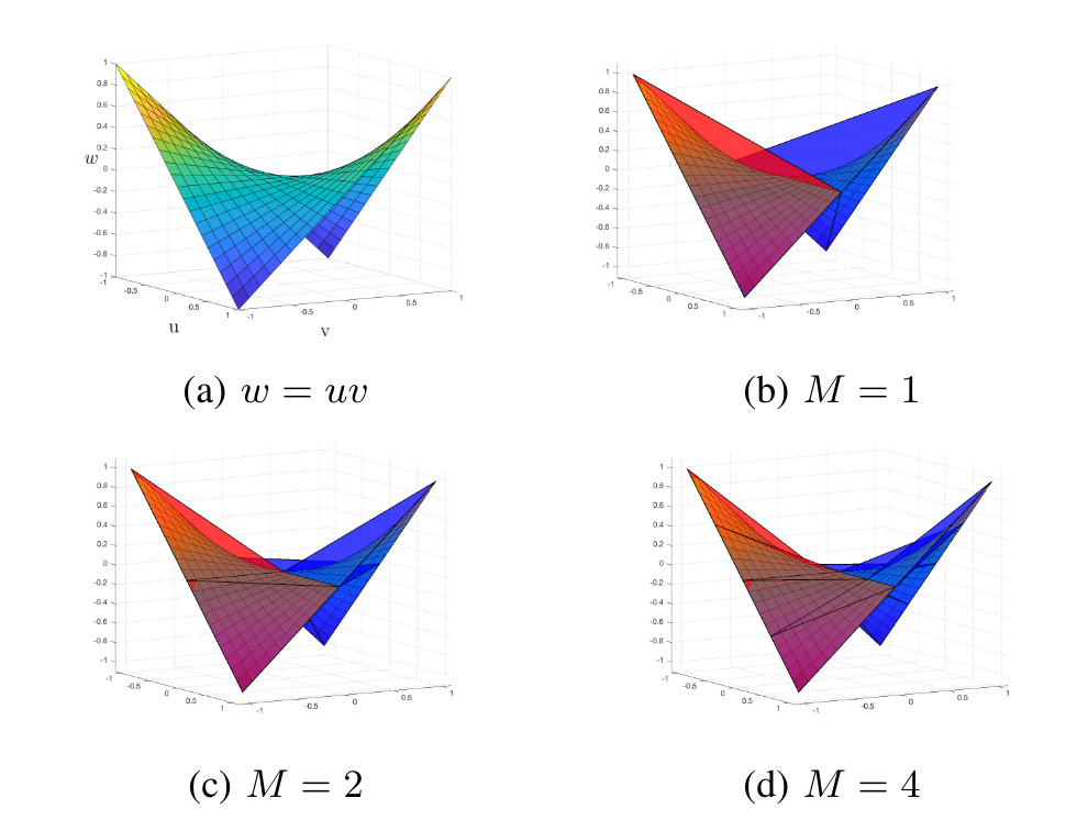
Solving it: SDP Relaxation

We solve it with the standard SDP relaxation

\begin{aligned} \min_{x} \quad \langle Q_0, X \rangle & \\ \text{subject to} \quad \langle Q_i, X \rangle &\geq 0, \quad \forall i = 1, \ldots \\ \quad AXA^\intercal &\geq 0 \\ \quad AXe_1^\intercal &\geq 0 \\ \quad e_1^\intercal X e_1 &= 1 \\ \quad X \succeq 0 \\ \end{aligned}

$ \longrightarrow $

Exact when $ \text{rank}(X) = 1 \iff X = x x^\intercal $
(This includes the McCormick envelope/outer-approximation of bilinear constraints)
Now we have a convex set!

$ X := xx^\intercal $

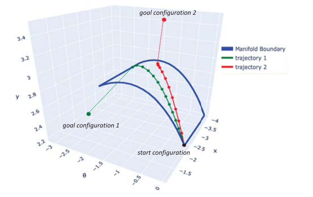
Minimizing kinetic energy makes the SO(2) relaxation tight

\begin{aligned} \min_{x_k \in \mathbb{R}^2} \quad & \sum^{d-1}_{k = 0} (x_{k+1} - x_{k})^\intercal (x_{k+1} - x_{k}) \\ \textrm{s.t.} \quad & x_k^\intercal x_k = 1 \quad k = 0, \ldots, d \\ \quad & x_0 = \bar x_I \\ \quad & x_d = \bar x_F \\ \end{aligned}

Formulate the following minimal problem

Solving the relaxed problem gives the true solution!
We expect this to also hold for SO(3)
(A formal tightness proof using the dual of the relaxation is in the works)

\begin{aligned} x_k &= \begin{bmatrix} \cos\theta_k \\ \sin\theta_k \\ \end{bmatrix} \\ &:= \begin{bmatrix} c_k \\ s_k \end{bmatrix}, \quad k = 0, \ldots, d \end{aligned}

Minimizing kinetic energy makes the SO(2) relaxation tight

Naive SOCP relaxation
$ c_\theta^2 + s_\theta^2 \leq 1 $

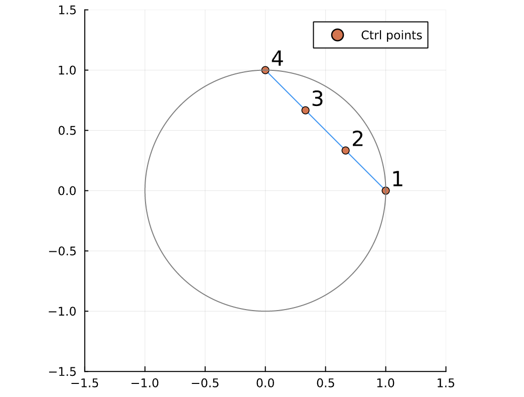
SDP relaxation

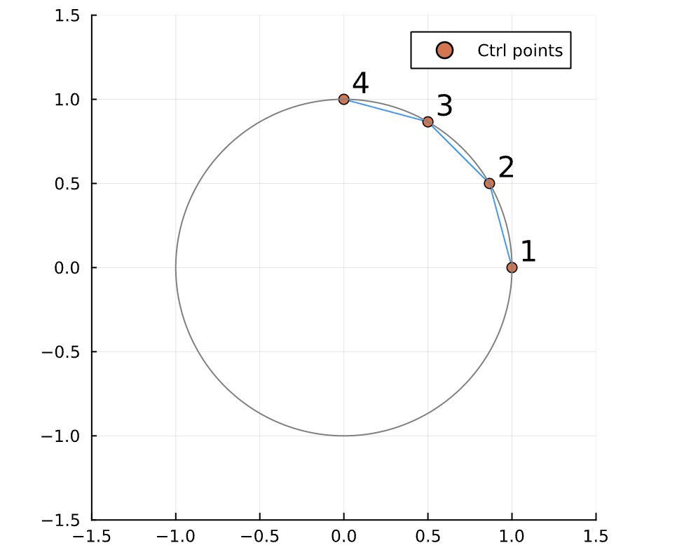
(Points 1 and 4 are fixed from boundary conditions)

Results

Making the contact modes convex

Object Flip-Ups & Pushing

Tightness Results

Pentagon

Mass: 1kg

COM to vertex: 0.2 m

"Reference force" = $ mg \approx 10 N $

Object Flip-Ups & Pushing

Tightness Results

Box

Mass: 1kg

COM to vertex: 0.2 m

"Reference force" = $ mg \approx 10 N $

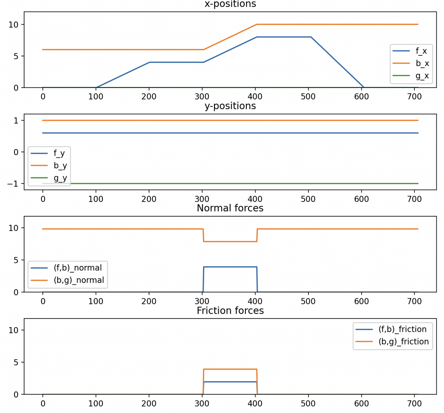
Object Flip-Ups & Pushing

Tightness Results

Worst case: Triangle

Mass: 1kg

COM to vertex: 0.2 m

"Reference force" = $ mg \approx 10 N $

Object Flip-Ups & Pushing

Tightness Results

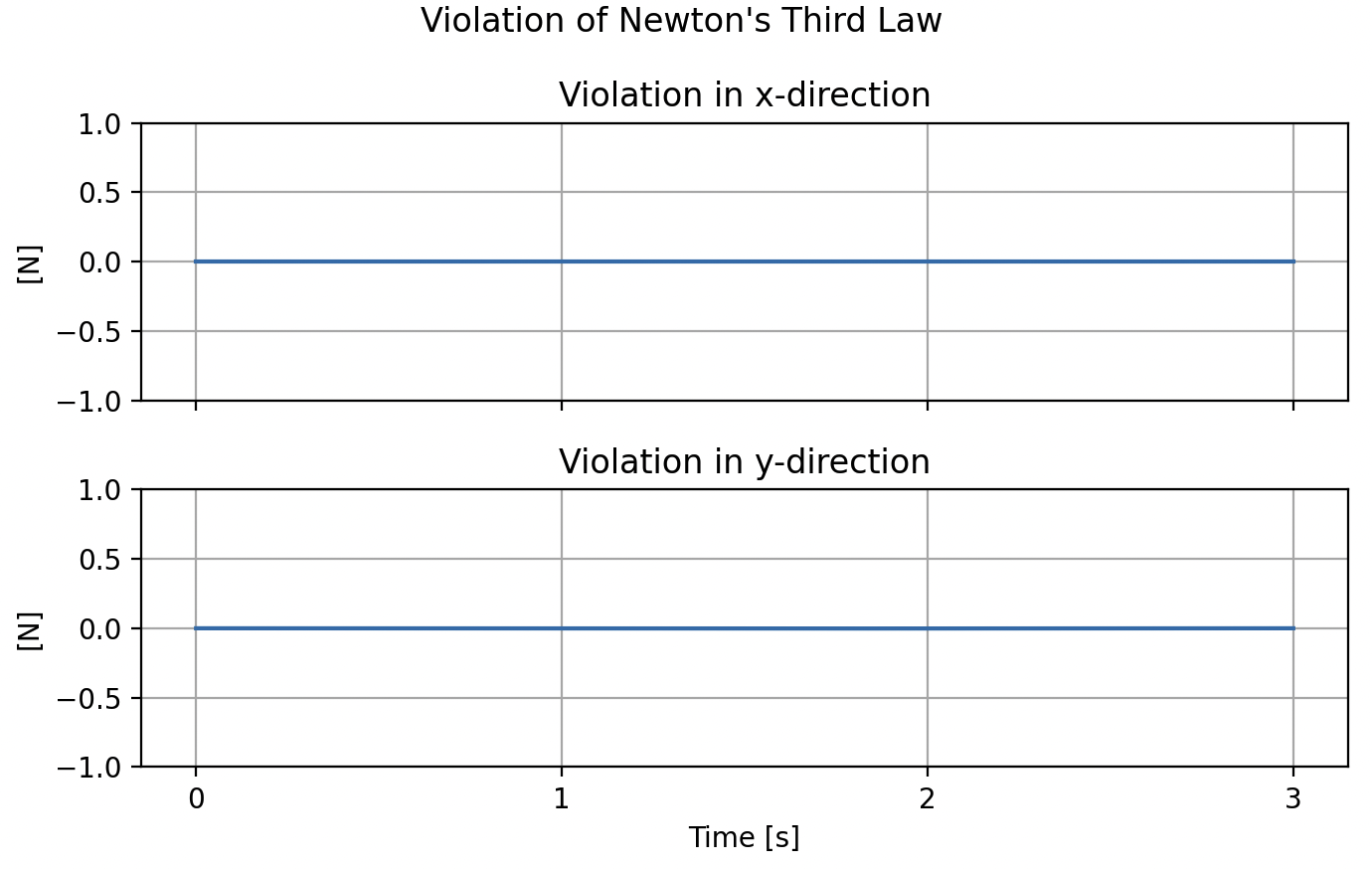
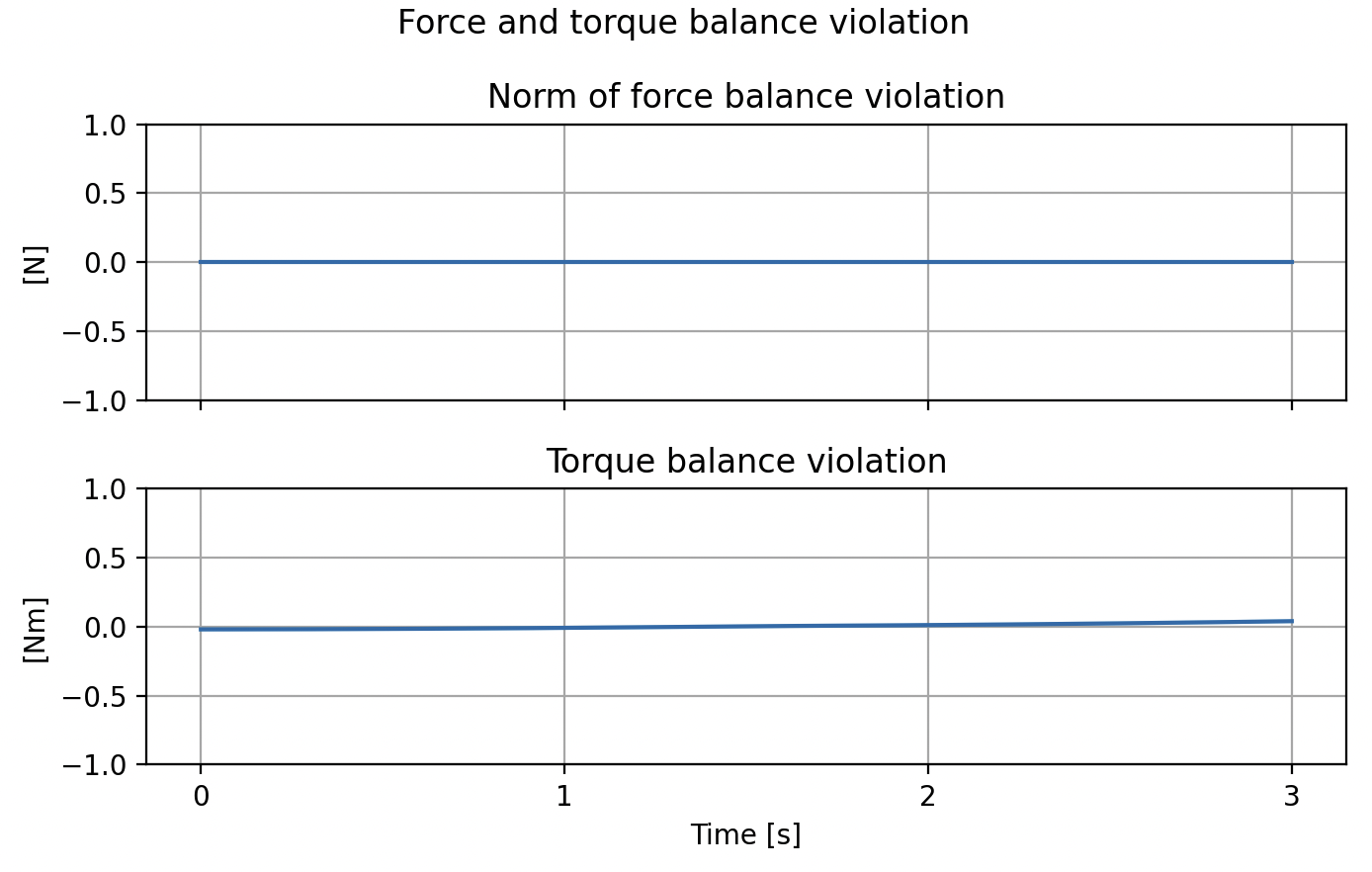
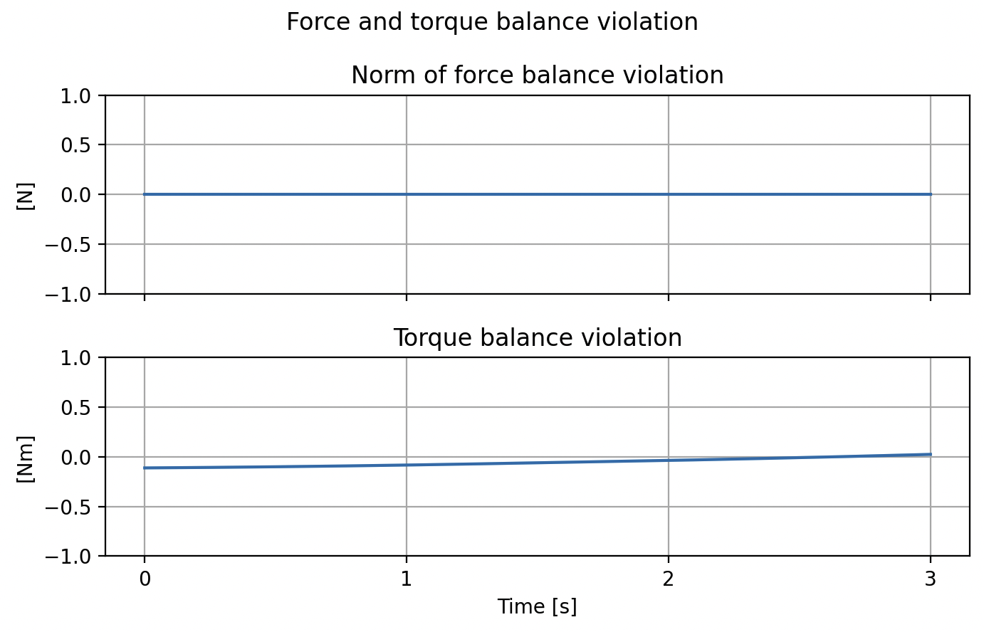
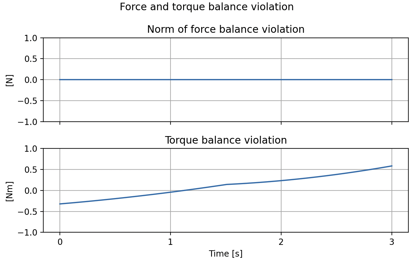
Preliminary Conclusions

SO(2) relaxation is tight
$ \implies $ Force balance is tight
Sometimes (small) violation of torque balance
For certain initial conditions, Newton's third law gets violated
(we suspect this is for infeasible initial conditions)

Planar Pushing

Tightness Results

For triangle:

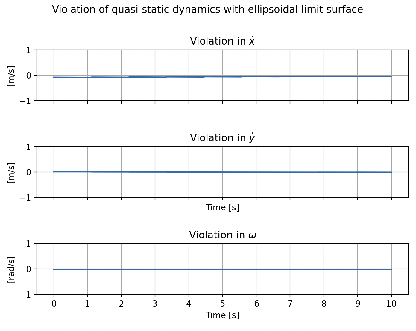
Similar for all shapes
Preliminary analysis: Seems to be tight

Future/planned work

Use GCS to plan through contact modes
Stabilize trajectories in simulation
Extend to the 3D case
Longer-term: Work on dealing with contact mode explosion