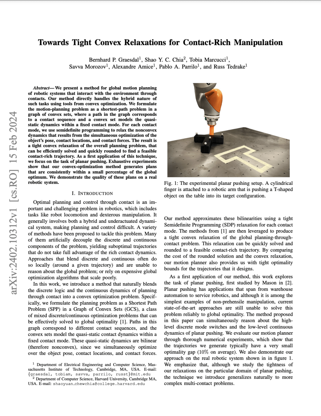
Towards Tight Convex Relaxations for Contact-Rich Manipulation
April 1st 2024
Bernhard Paus Graesdal
ONR Autonomy Project: Pieter, Russ, Stephen, Zico
Motivation
- Optimal planning through contact is hard
- Generally both a hybrid and underactuated system
- Existing methods often artificially decouple continuous and discrete part of the problem
Goal
A method that blends discrete logic and continuous dynamics to leverage the rich contact dynamics
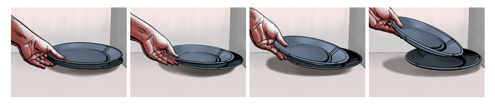
Example tasks
C. Chi et al., “Diffusion Policy: Visuomotor Policy Learning via Action Diffusion.” Mar. 09, 2023
- How do we plan for such tasks?
N. Doshi et al., “Manipulation of unknown objects via contact configuration regulation.” Jun. 01, 2022
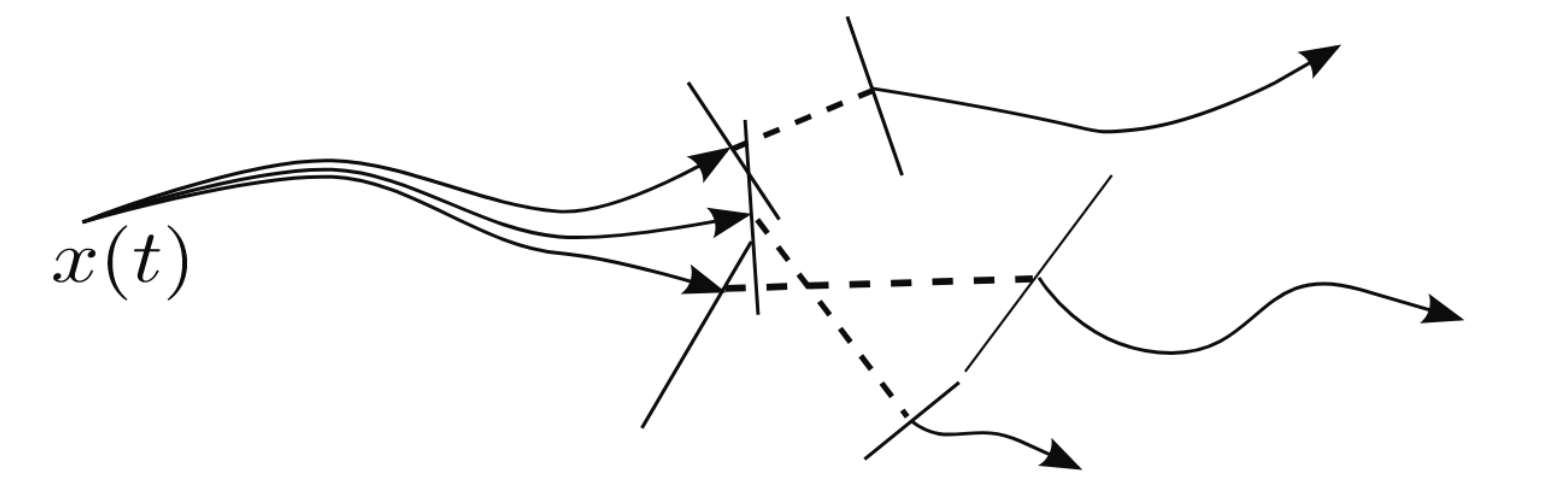
High-Level Approach
- Formulate the problem as a Shortest Path Problem in a Graph of Convex Sets (GCS)
- Paths in the graph: Different contact sequences
- Convex sets: Model contact dynamics
- A point in a convex set \(\iff\) A trajectory within a fixed contact mode
- A feasible GCS path corresponds to a contact trajectory
\(\iff\)

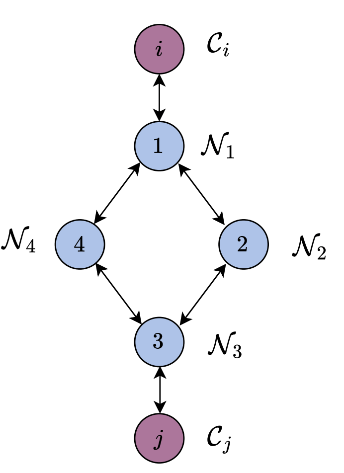
Graphs of Convex Sets

-
For each \(i \in V:\)
- Compact convex set \(X_i \subset \R^d\)
- A point \(x_i \in X_i \)
- Vertex cost given by a convex function \[ \ell_v(x_i) \]
- New machinery to tighten convex relaxation
Note: The blue regions are not obstacles.
Novelty in our method
- Leverage a tight convex relaxation for the (nonconvex) bilinearities in each contact mode
- Use GCS machinery to produce a tight convex relaxation for the global planning-through-contact problem
- Obtain near-globally optimal solutions by solving a single SDP followed by a quick rounding step

- As a first step, we apply our method to planar pushing
- The approach generalizes to more complex contact-rich tasks
Planar Pushing
- Goal: Manipulate object to target pose
- One of the simplest examples of non-prehensile manipulation
- Still state-of-the-art are unable to reliably solve to global optimality
- Our method will:
- Plan a (close to) globally optimal contact-rich trajectory for manipulating the object to its target pose
- While simultaneously planning the collision-free motion between contacts
Dynamics of Planar Pushing
- Hybrid dynamical system:
- Contact and non-contact modes
- Assume quasi-static dynamics, low velocities, no work done by impacts
- Simultaneously optimize over poses and contact forces
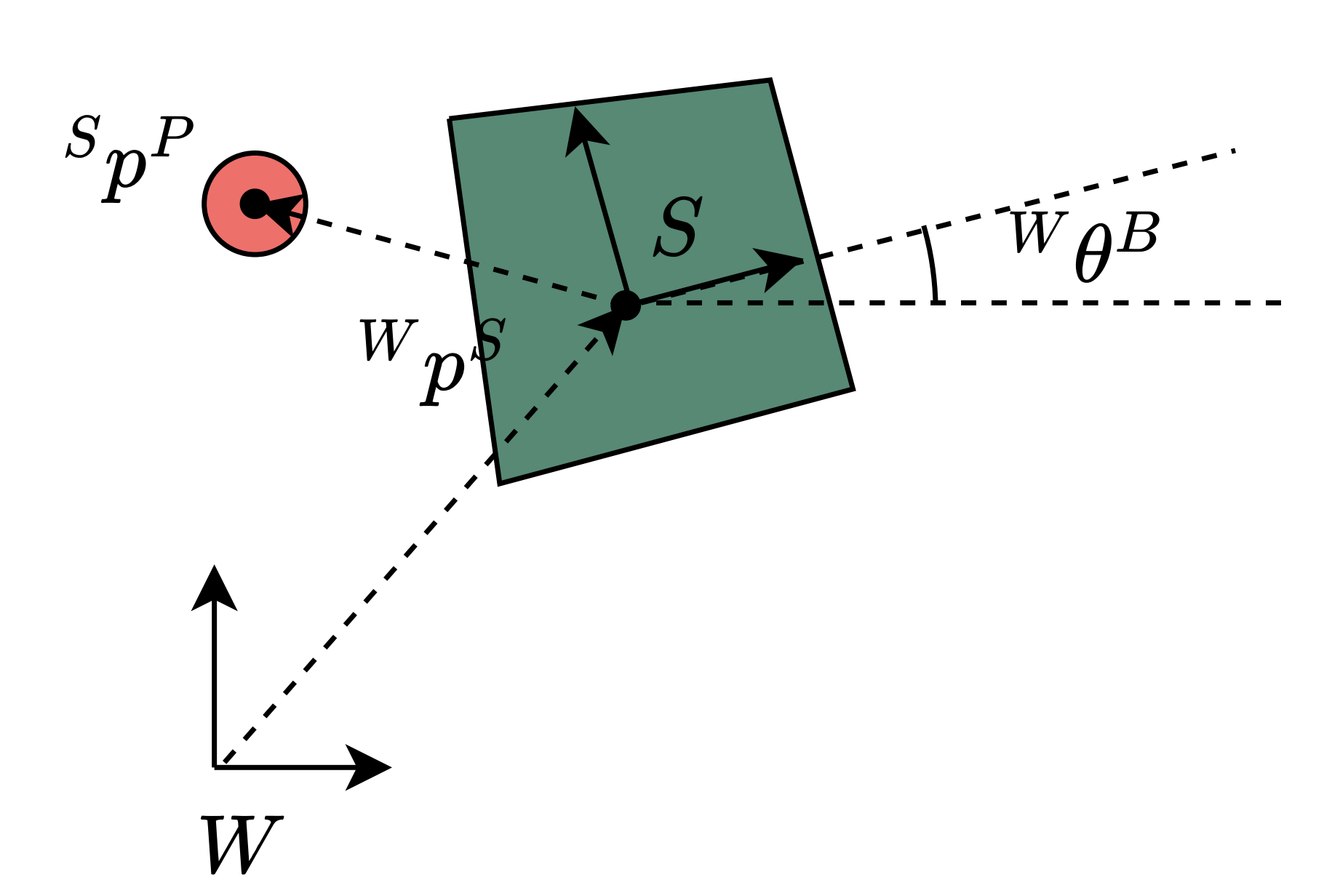
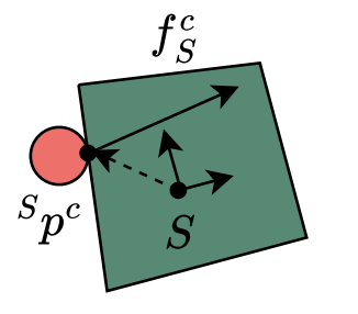
Mode class 1: Contact between the pusher and a face of the slider
- Bilinear (non-convex) dynamics due to:
- Rotation membership in \( \text{SO}(2) \)
- Cross-product between contact point and contact force (torque) in rotational dynamics
- Rotation of forces between frames in dynamics
- All can be represented with quadratic equality constraints (non-convex)
Dynamics of Planar Pushing
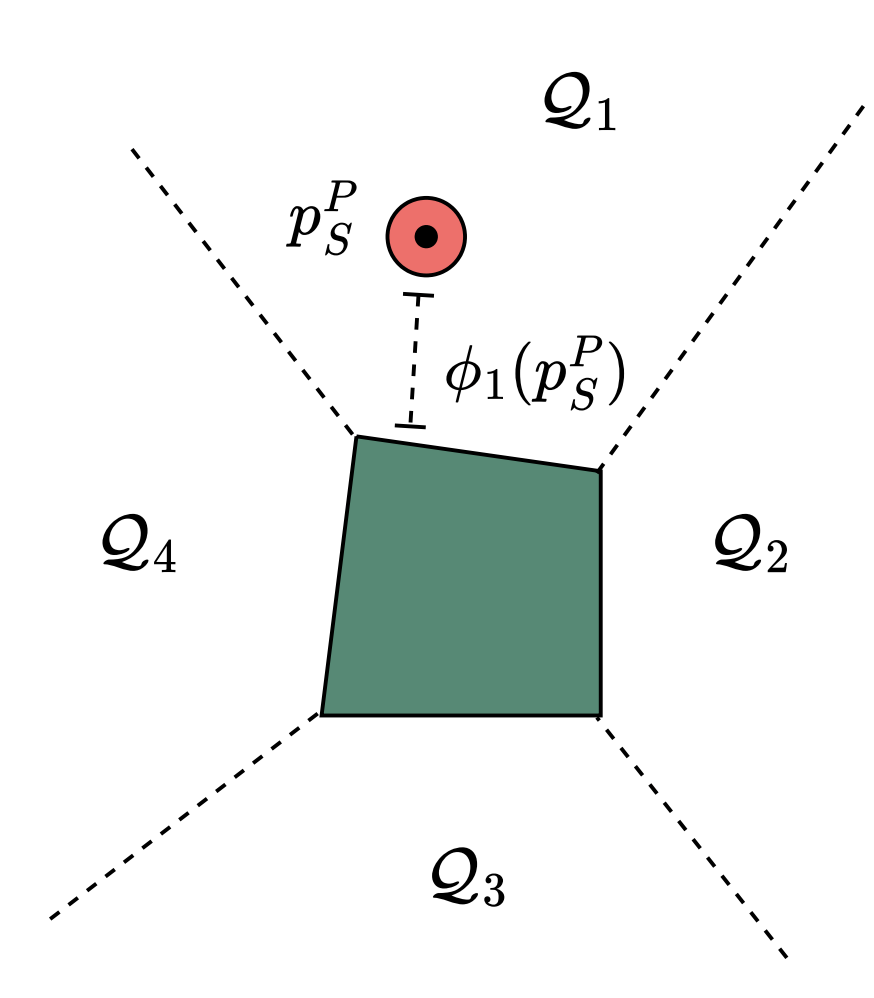
Mode class 2: Non-contact
- We decompose the collision-free space (similar to GCSTrajOpt) in task space
- Piecewise linear approximation of SDF in each region
- With this we can encode planning for non-contact modes as a convex problem

Dynamics of Planar Pushing
Semidefinite Relaxation of contact modes
Motion planning in a contact mode can be formulated in the form:
where \(Q_i\) possibly indefinite, hence problem is nonconvex
Lift the problem:
\( x \in \R^n \rightarrow (x, X) \in \R^n \times \mathbb{S}^{n \times n}\)
Equivalent when \( \text{rank}(X) = 1 \iff X = x x^\intercal \)
Otherwise a convex relaxation
\( \longrightarrow \)
\( X := xx^\intercal \)
Semidefinite Relaxation of contact modes
- Tightening constraints: \( A X A^T \geq 0 \) is implied by \(Ax \geq 0\) and potentially tightens the formulation
- We have done work on finding additional tightening constraints
- Multiply quadratic constraints that simplify to new quadratic constraints (i.e. we can still use the first-order SDP relaxation!)
- Enforce the dynamics in both frames:
\( v = R u \iff R^T v = u \) is implied by \(R^T R = I\)
Motion Planning as Graph Search
- We will "Add the modes to the graph" = Add a vertex with the feasible set as the convex set and the cost as the vertex cost
- Idea: Build a graph of convex sets to represent the motion planning problem
- Planning within each fixed mode can be formulated as a convex program
Motion Planning as Graph Search
- Add a contact mode for each face of the object
- Encode collision-free motion planning between contacts: Transition through non-contact modes
- This allows transitions from any face to any face
- Allows at most one visit with a fixed horizon length to each face: can repeat the vertices in the graph to have more
- Initial and target poses as source and target (singleton) vertices in the graph
How to structure the graph and mode transitions?
\(\updownarrow\)
The motion planning algorithm
- Solve SPP in GCS problem
- Use flows as probabilities and sample N paths
- For each path: round to feasibility by solving a cheap nonlinear program from relaxed solution
- Pick the trajectory with the lowest cost
- Most expensive part is the first SDP: everything else is very cheap!
- We also get an upper bound on global optimality gap:
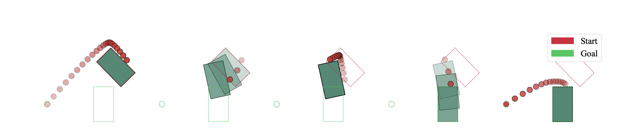
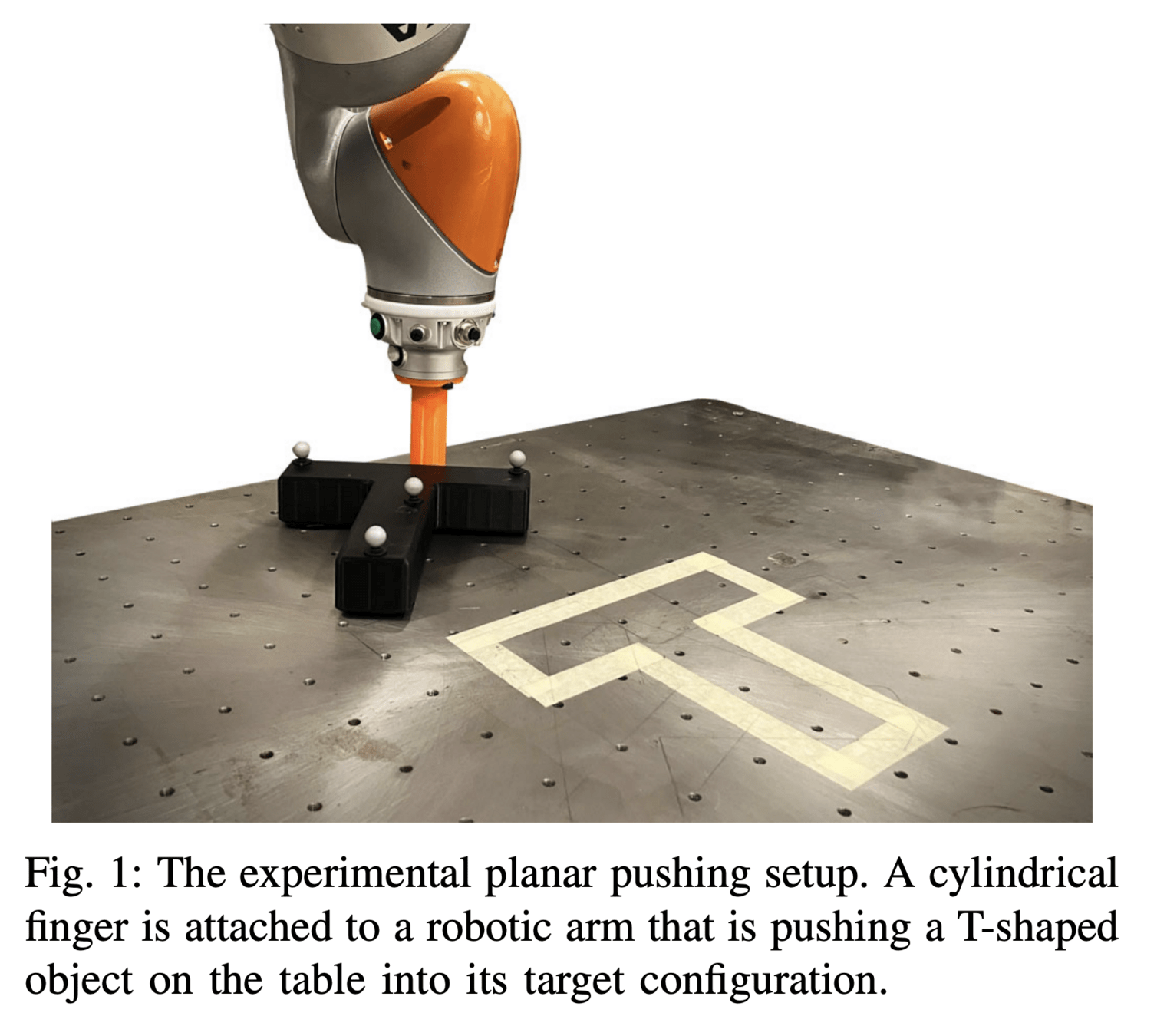
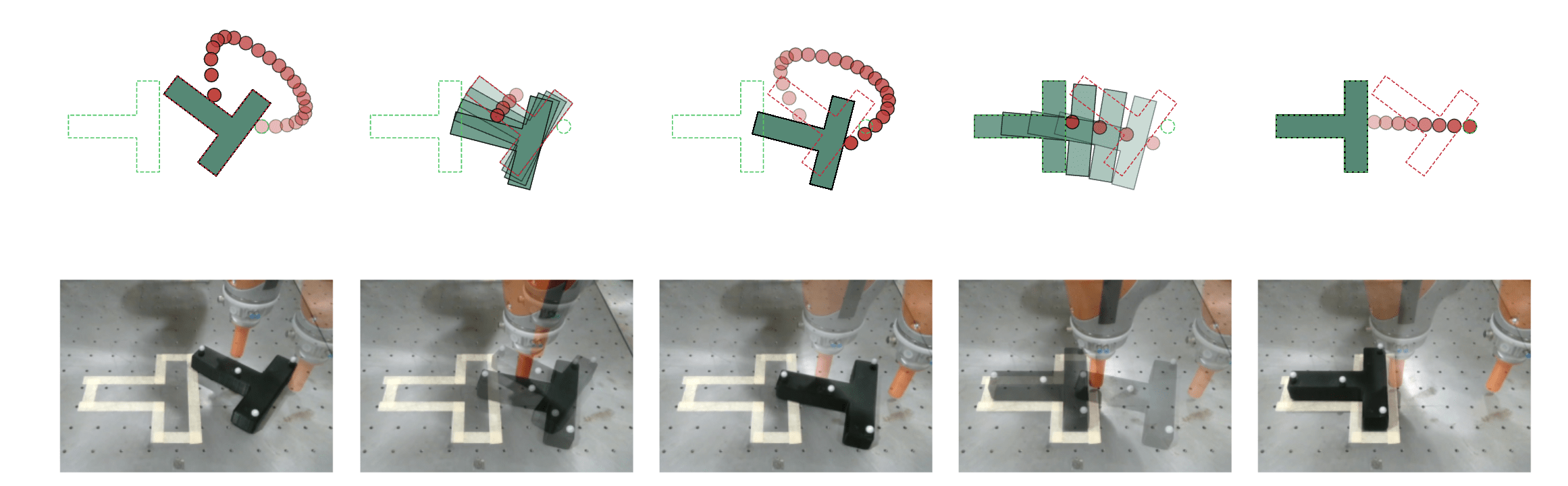
Results
Hardware experiments
(4x is due to MIQP feedback controller)
Numerical results
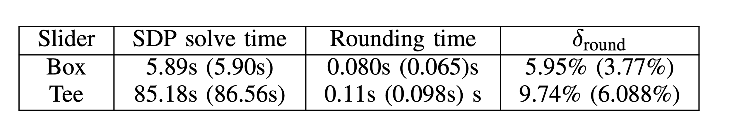
- Consistently within a small percentage of global optimum
- Solve times a few seconds for the box, 1.5 minutes for the Tee (box has 4 faces, tee has 8 faces)
- Expensive part is solving the big SDP. Rounding is very cheap!
- For comparison: enumerating all mode sequences and solving nonlinear program would take \( 8! \times 0.1 s \approx 67\) minutes (assuming the nonlinear program always gave a good solution)
(Reported values are mean values, with median in parenthesis)
Numerical results
- We have not yet compared to MINLP which we will do for the paper rebuttal
(Reported values are mean values, with median in parenthesis)
Preprint available on Arxiv: https://arxiv.org/abs/2402.10312
Future directions...
Policy
Training
Data
Trajectory Generation
GCS \( \rightarrow \) BC w/ Diffusion Policy
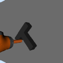
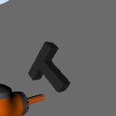
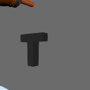
Example: Push-T Task (with Kuka)

- Use GCS for data generation
\(\rightarrow\) Train BC policy directly on data
Adam Wei
Planning through contact for general manipulation

- Addresses scalability by avoiding explicit enumeration of contact modes
- Plan: Decompose the space into convex regions and use GCS to plan through these