Topic Modeling
Latent Dirichlet Allocation
Each document is a mixture of topics.
LDA
Each topic is a probability distribution over words.
1
2
two simple assumptions:
slide 1
LDA
1
2
slide 1
Each document is a mixture of topics.
Each topic is a probability distribution over words.
Latent Dirichlet Allocation
LDA
1
2
slide 1
Each document is a mixture of topics.
Each topic is a probability distribution over words.
Latent Dirichlet Allocation
LDA
1
2

deer-in-a-chalet
slide 1
Each document is a mixture of topics.
Each topic is a probability distribution over words.
Latent Dirichlet Allocation
-
For each topic \( k \)
- draw a word distribution \( \phi_k \sim Dir(\beta) \)
-
For each document \( d \)
- draw a topic distribution \( \theta \sim Dir(\alpha) \)
-
For each of the \( N \) words \( w_n \):
- Choose a topic \( z_n \sim Multinomial (\theta) \)
- Choose a word \( w_n \sim Multinomial (\phi) \)
\( \alpha \)
\( \theta \)
\( z \)
\( w\)
\( \beta \)
\( M \)
\( N \)
Generative Process
\( \phi \)
\( K \)

slide 2
A probabilistic story how text could have been generated.
Example
election
election
ballot
ballot
quantum
quantum
quantum
quantum
basketball
election
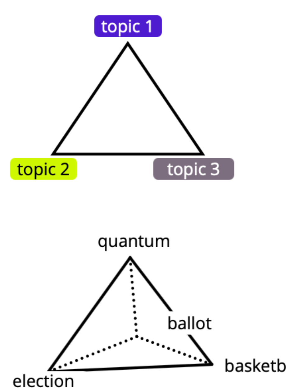
Topics
topic 1
topic 2
topic 3
Words
election
ballot
quantum
basketball
slide 3
Words
election
ballot
quantum
basketball
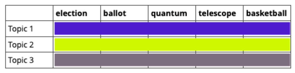
Each topic is a probability distribution over words.
slide 3
election
ballot
quantum
basketball
-
Dirichlet Prior:
- Each topic is primarily associated with one word.
slide 3
election
ballot
quantum
basketball
election |
ballot |
quantum |
basketball |
|
|---|---|---|---|---|
Topic 1 |
0.4 |
0.4 |
0.1 |
0.1 |
Topic 2 |
0.1 |
0.1 |
0.75 |
0.05 |
Topic 3 |
0.1 |
0.1 |
0.05 |
0.75 |
slide 3
Words
election
ballot
quantum
basketball
slide 3
Words
election
ballot
quantum
basketball
Topics
topic 1
topic 2
topic 3
election
election
ballot
ballot
quantum
quantum
quantum
quantum
basketball
election
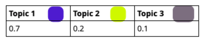
Each document is a mixture of topics.
slide 3
-
Dirichlet Prior:
- Each document is primarily about one topic.
topic 1
topic 2
topic 3
slide 3
topic 1
topic 2
topic 3
Topic 1 |
Topic 2 |
Topic 3 |
|---|---|---|
0.7 |
0.2 |
0.1 |
Topic 1 |
Topic 2 |
Topic 3 |
|---|---|---|
0.2 |
0.7 |
0.1 |
slide 3
slide 4
\( \alpha \)
\( \theta \)
\( z \)
\( w\)
\( \beta \)
\( M \)
\( N \)
\( \phi \)
\( K \)
election
document-topic distribution
word-topic distribution
LDA Generative Process
slide 4
\( \alpha \)
\( \theta \)
\( z \)
\( w\)
\( \beta \)
\( M \)
\( N \)
\( \phi \)
\( K \)
election
word-topic distribution
election
ballot
ballot
quantum
slide 5
Initial Random Allocation
topic 1
topic 2
topic 3
slide 5
topic 1
topic 2
topic 3
quantum
basketball
election
ballot
Initial Random Allocation
We want
- documents to become thematically coherent, and
- topics to become semantically focused.
slide 5
topic 1
topic 2
topic 3
quantum
basketball
election
ballot
- We cannot compute these positions analytically.
- LDA uses approximate inference,
typically Gibbs sampling.
slide 5
Appendix
Outlook
In 2003, LDA was groundbreaking
It was unsupervised (no labeled data was needed).
-
It provided interpretable topics.
-
It was efficient for small to medium-sized datasets.
Limitations of LDA
-
Bag-of-Words Assumption – It ignores word order.
-
The number of topics needs to be pre-specified.
-
LDA struggles with very large datasets.
Choosing a Topic Modeling Approach
-
Today, transformer-based models offer more advanced topic modeling.
-
BERTopic clusters transformer-generated sentence embeddings.
-
These capture semantics better than LDA, providing more meaningful topics.
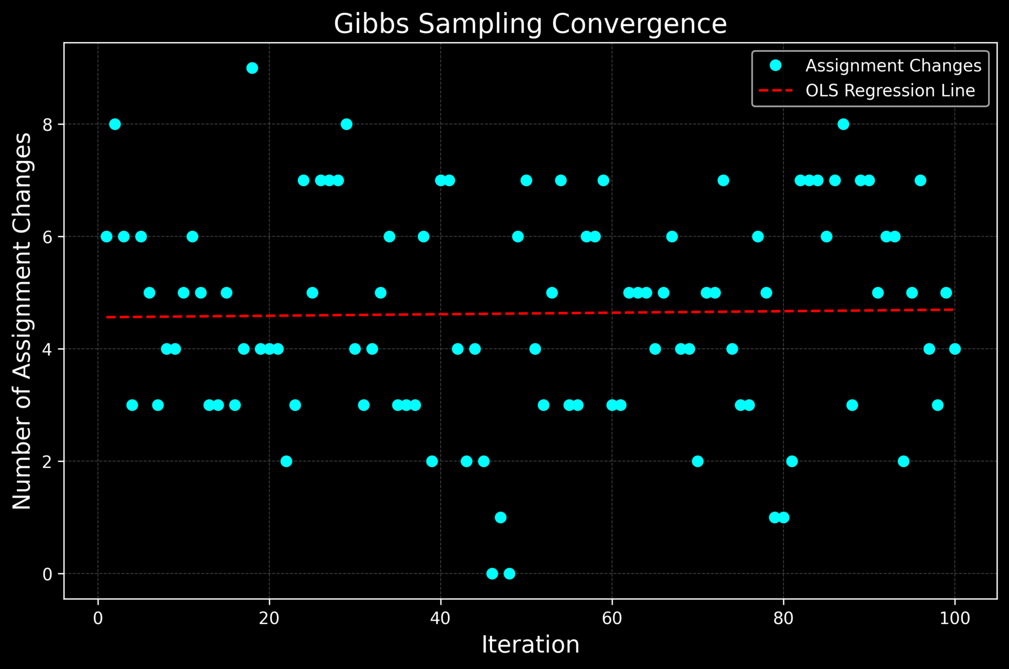
A Challenge For You
Our Gibbs Sampler does not converge.
Work in pairs to achieve convergence!
import numpy as np
import pandas as pd
import matplotlib.pyplot as plt

# For reproducibility
np.random.seed(42)

#############################
# 1. SETUP
#############################
topics = ["politics", "science", 'sports']
vocab = ["election", "ballot", "quantum", "basketball"]
V = len(vocab)
K = len(topics)
D = 2

# Hyperparameters for Dirichlet distributions
alpha = np.array([0.5, 0.5, 0.5])  # Prior for document-topic distribution (θ) #TRY
beta = np.ones(V) * 5  # Prior for topic-word distribution (ϕ) #TRY

#############################
# 2. Generate Topic-Word Distributions (ϕ)
#############################
# Each topic's word distribution is sampled from a Dirichlet with parameter beta.
phi = np.array([np.random.dirichlet(beta) for _ in range(K)])
print("Topic-word distributions (phi):")
for i, row in enumerate(phi):
    print(f"{topics[i]}: " + " ".join(f"{x:.2f}" for x in row))

#############################
# Documents that I have (e.g. real documents downloaded from a newspaper site)
# THIS IS THE REAL TRUE HIDDEN ASSIGNMENT
#############################
documents = [
    [('election', 'politics'), ('election', 'politics'), ('ballot', 'politics'), ('ballot', 'politics'), ('quantum', 'science')],
    [('quantum', 'science'), ('quantum', 'science'), ('quantum', 'science'), ('basketball', 'sports'), ('election', 'politics')]
]

# Sample topic distribution for each document from Dirichlet(alpha)
theta = np.array([np.random.dirichlet(alpha) for _ in range(D)])

# Sample a topic for the word based on theta[d]
sampled_documents = []
for d in range(D):
    sampled_doc = []
    for word, _ in documents[d]:  # Ignore the true hidden assignment
        topic_idx = np.random.choice(K, p=theta[d])
        sampled_topic = topics[topic_idx]
        sampled_doc.append((word, sampled_topic))
    sampled_documents.append(sampled_doc)

df_sampled_documents = {
    f"Doc {d + 1}": pd.DataFrame(sampled_documents[d], columns=["Word", "Sampled Topic"])
    for d in range(D)
}
df_sampled_documents

#############################
# 4. INITIALIZE COUNT MATRICES FOR GIBBS SAMPLING
#############################
doc_topic_counts = np.zeros((D, K)) # for each document
word_topic_counts = np.zeros((K, V)) # for all documents
documents_assignments = []

for d, doc in enumerate(documents):
    doc_assignments = []
    for word, assigned_topic in doc:
        topic_idx = topics.index(assigned_topic)
        word_idx = vocab.index(word)
        doc_topic_counts[d, topic_idx] += 1
        word_topic_counts[topic_idx, word_idx] += 1
        doc_assignments.append(topic_idx)
    documents_assignments.append(doc_assignments)

pd.DataFrame(doc_topic_counts, index=["Doc 1", "Doc 2"], columns=["politics", "science", "sport"])
pd.DataFrame(word_topic_counts, index=["politics", "science", 'sports'], columns=["election", "ballot", "quantum", "basketball"])


#############################
# 5. GIBBS SAMPLING OVER ALL DOCUMENTS
#############################
num_iterations = 100  #TRY
changes_history = []

for it in range(num_iterations):
    total_changes = 0
    for d, doc in enumerate(documents):
        for i, (word, _) in enumerate(doc):
            current_topic = documents_assignments[d][i]
            word_idx = vocab.index(word)

            # Remove the current assignment (the "minus i" counts)
            doc_topic_counts[d, current_topic] -= 1
            word_topic_counts[current_topic, word_idx] -= 1

            # Compute the conditional probability for each topic
            topic_probs = np.zeros(K)
            for k in range(K):
                # Component from document-topic: how many times topic k appears in document d (plus alpha)
                doc_prob = doc_topic_counts[d, k] + alpha[k]
                # Component from topic-word: how likely word appears in topic k
                word_prob = (word_topic_counts[k, word_idx] + beta[word_idx]) / (
                            np.sum(word_topic_counts[k]) + np.sum(beta))
                topic_probs[k] = doc_prob * word_prob

            # Normalize to form a valid probability distribution
            topic_probs = topic_probs / np.sum(topic_probs)

            # Sample a new topic based on computed probabilities
            new_topic = np.random.choice(K, p=topic_probs)

            # Check if the assignment has changed
            if new_topic != current_topic:
                total_changes += 1

            # Update counts with the new assignment
            doc_topic_counts[d, new_topic] += 1
            word_topic_counts[new_topic, word_idx] += 1
            documents_assignments[d][i] = new_topic

    changes_history.append(total_changes)
    print(f"\nIteration {it + 1}: Number of topic assignment changes = {total_changes}")
    print("Document-topic counts:")
    print(doc_topic_counts)
    print("Word-topic counts:")
    print(word_topic_counts)


x = np.arange(1, num_iterations + 1)
y = np.array(changes_history)
slope, intercept = np.polyfit(x, y, 1)
reg_line = slope * x + intercept


plt.style.use("dark_background")
plt.figure(figsize=(10, 6))
plt.plot(x, y, marker='o', linestyle='', color='cyan', label='Assignment Changes')
plt.plot(x, reg_line, 'r--', label='OLS Regression Line')
plt.xlabel("Iteration", fontsize=14, color="white")
plt.ylabel("Number of Assignment Changes", fontsize=14, color="white")
plt.title("Gibbs Sampling Convergence", fontsize=16, color="white")
plt.legend()
plt.grid(color="gray", linestyle="--", linewidth=0.5, alpha=0.5)
plt.savefig("plots/gibbs_sampling_convergence.png", dpi=300, bbox_inches="tight", facecolor="black")
plt.show()
Happy Modeling!
-
Blei, David M., Andrew Y. Ng, and Michael I. Jordan.
"Latent dirichlet allocation."
Journal of machine Learning research 3. Jan (2003): 993-1022.
-
Jurafsky, Daniel.
"Speech and language processing." (2025).
-
Quinn, Kevin M., et al.
"How to analyze political attention with minimal assumptions and costs."
American Journal of Political Science 54.1 (2010): 209-228.
Further Reading
BERTopic
Transformer-Based Topic Modeling
-
Generate Embeddings: Uses BERT/SBERT/RoBERTa to create dense vector representations for each document.
-
Dimensionality Reduction: Applies UMAP to reduce embeddings while preserving local structure.
-
Clustering: Uses HDBSCAN to group similar documents into topics.
-
Topic Representation: Uses class-based TF-IDF to extract the most representative words per topic.
A common goal is to summarize or classify documents based on their content.

Why start with LDA in 2026?
LDA remains foundational because it introduced the core grammar of modern topic modeling:
- Latent variables: topics as unobserved structure
- Mixed membership: documents as topic distributions
- Approximate inference: Gibbs / variational methods
- Generative modeling: explicit assumptions about text
Modern approaches (neural topic models, BERTopic, embeddings) change the machinery — not the underlying problem:
- How do we infer latent thematic structure from text under uncertainty?
from gensim.models import LdaModel


documents = [
    "Die Regierung plant eine neue Steuerreform und diskutiert sie im Bundestag.",
    "Der Kanzler spricht über die wirtschaftliche Lage und neue Gesetze.",
    "Im Parlament gibt es eine Debatte über soziale Gerechtigkeit und Mindestlohn.",
    "Die globale Erwärmung bedroht unser Klima. Wissenschaftler fordern Maßnahmen.",
    "Klimaschutz ist wichtig. Neue CO2-Gesetze sollen die Umwelt verbessern."
]

dictionary = corpora.Dictionary(documents)


lda_model = LdaModel(documents,
                     num_topics = 2)  # You choose the number of topics to extract!
Topic 1: 0.3 klima + 0.25 co2 + 0.20 umwelt + 0.15 erwärmung
Topic 2: 0.35 regierung + 0.30 bundestag + 0.20 kanzler + 0.15 parlament
Climate Change
Politics
Publication: Journal of Machine Learning Research 3/2003
How does LDA uncover meaningful topics without knowing the meaning of words?
Topic 1 |
Topic 2 |
Topic 3 |
|---|---|---|
0.7 |
0.2 |
0.1 |
Topic 1 |
Topic 2 |
Topic 3 |
|---|---|---|
0.2 |
0.7 |
0.1 |
slide 3
Topic Assignment Process
election election ballot
ballot
quantum
quantum
quantum
quantum
basketball
election
Topic 1 |
Topic 2 |
Topic 3 |
|---|---|---|
0.7 |
0.2 |
0.1 |
Topic 1 |
Topic 2 |
Topic 3 |
|---|---|---|
0.2 |
0.7 |
0.1 |
slide 3
Topic Assignment Process
election election ballot
ballot
quantum
quantum
quantum
quantum
basketball
election
Topic 1 |
Topic 2 |
Topic 3 |
|---|---|---|
0.7 |
0.2 |
0.1 |
Topic 1 |
Topic 2 |
Topic 3 |
|---|---|---|
0.2 |
0.7 |
0.1 |
slide 3
Topic Assignment Process
election election ballot
ballot
quantum
quantum
quantum
quantum
basketball
election
Topic 1 |
Topic 2 |
Topic 3 |
|---|---|---|
0.7 |
0.2 |
0.1 |
Topic 1 |
Topic 2 |
Topic 3 |
|---|---|---|
0.2 |
0.7 |
0.1 |
slide 3
Topic Assignment Process
election election ballot
ballot
quantum
quantum
quantum
quantum
basketball
election
Topic 1 |
Topic 2 |
Topic 3 |
|---|---|---|
0.7 |
0.2 |
0.1 |
Topic 1 |
Topic 2 |
Topic 3 |
|---|---|---|
0.2 |
0.7 |
0.1 |
slide 3
Topic Assignment Process
election election ballot
ballot
quantum
quantum
quantum
quantum
basketball
election
Topic 1 |
Topic 2 |
Topic 3 |
|---|---|---|
0.7 |
0.2 |
0.1 |
Topic 1 |
Topic 2 |
Topic 3 |
|---|---|---|
0.2 |
0.7 |
0.1 |
slide 3
Topic Assignment Process
election election ballot
ballot
quantum
quantum
quantum
quantum
basketball
election
Topic 1 |
Topic 2 |
Topic 3 |
|---|---|---|
0.7 |
0.2 |
0.1 |
Topic 1 |
Topic 2 |
Topic 3 |
|---|---|---|
0.2 |
0.7 |
0.1 |
slide 3
Topic Assignment Process
election election ballot
ballot
quantum
quantum
quantum
quantum
basketball
election
Topic 1 |
Topic 2 |
Topic 3 |
|---|---|---|
0.7 |
0.2 |
0.1 |
Topic 1 |
Topic 2 |
Topic 3 |
|---|---|---|
0.2 |
0.7 |
0.1 |
slide 3
Topic Assignment Process
election election ballot
ballot
quantum
quantum
quantum
quantum
basketball
election
Topic 1 |
Topic 2 |
Topic 3 |
|---|---|---|
0.7 |
0.2 |
0.1 |
Topic 1 |
Topic 2 |
Topic 3 |
|---|---|---|
0.2 |
0.7 |
0.1 |
slide 3
Topic Assignment Process
election election ballot
ballot
quantum
quantum
quantum
quantum
basketball
election
slide 3
election election ballot
ballot
quantum
quantum
quantum
quantum
basketball
election
topic 1 |
topic 2 |
topic 3 |
|
|---|---|---|---|
doc 1 |
3 |
1 |
1 |
doc 2 |
2 | 2 | 1 |
count
Initial random allocation
of topics to words.
election |
ballot |
quantum |
basketball |
|
|---|---|---|---|---|
topic 1 |
1 |
1 |
2 |
0 |
topic 2 |
1 |
1 |
1 |
1 |
topic 3 |
1 |
0 |
1 |
0 |
Gibbs Sampling
election election ballot
ballot
quantumtopic 1 |
topic 2 |
topic 3 |
|
|---|---|---|---|
doc 1 |
3 |
1 |
1 |
doc 2 |
1 |
3 |
1 |
Gibbs Sampling
election |
ballot |
quantum |
basketball |
|
|---|---|---|---|---|
topic 1 |
1 |
1 |
2 |
0 |
topic 2 |
1 |
1 |
1 |
1 |
topic 3 |
1 |
0 |
1 |
0 |
– 1
– 1
\( P(\text{election}|\text{topic 3}) = \frac{(0+0.01)}{(1 + 4 \times 0.01)} \approx 0.4 \)
\( \sum \) 1
\( \sum \) 4
election election ballot
ballot
quantumtopic 1 |
topic 2 |
topic 3 |
|
|---|---|---|---|
doc 1 |
3 |
1 |
1 |
doc 2 |
1 |
3 |
1 |
election |
ballot |
quantum |
basketball |
|
|---|---|---|---|---|
topic 1 |
1 |
1 |
2 |
0 |
topic 2 |
1 |
1 |
1 |
1 |
topic 3 |
1 |
0 |
1 |
0 |
– 1
– 1
\( \sum \) 3
\( P(\text{topic 3}|d) = \frac{(0 + 0.1)}{(5 + 3 \times 0.1)} \approx 0.23 \)
\( \sum \) 5
election election ballot
ballot
quantumtopic 1 |
topic 2 |
topic 3 |
|
|---|---|---|---|
doc 1 |
3 |
1 |
1 |
doc 2 |
1 |
3 |
1 |
election |
ballot |
quantum |
basketball |
|
|---|---|---|---|---|
topic 1 |
1 |
1 |
2 |
0 |
topic 2 |
1 |
1 |
1 |
1 |
topic 3 |
1 |
0 |
1 |
0 |
– 1
– 1
\( P(\text{election}|\text{topic 3}) = \frac{(0+0.01)}{(1 + 4 \times 0.01)} \approx 0.4 \)
\( P(\text{topic 3}|\text{election}) \approx 0.058\)
\( \times \)
\( \propto \)
\( P(\text{topic 3}|d) = \frac{(0 + 0.1)}{(5 + 3 \times 0.1)} \approx 0.23 \)
topic 1 |
topic 2 |
topic 3 |
|---|---|---|
0.058
0.064
0.24
election election ballot
ballot
quantumtopic 1 |
topic 2 |
topic 3 |
|---|---|---|
0.66 |
0.17 |
0.16 |
topic 1 |
topic 2 |
topic 3 |
|---|---|---|
0.058
0.064
0.24
normalize
election election ballot
ballot
quantumtopic 1 |
topic 2 |
topic 3 |
|---|---|---|
0.058 |
0.064
0.24
topic 1 |
topic 2 |
topic 3 |
|---|---|---|
0.66 |
0.17 |
0.16 |
election election ballot
ballot
quantumtopic 1 |
topic 2 |
topic 3 |
|
|---|---|---|---|
doc 1 |
3 |
1 |
0 |
doc 2 |
1 |
3 |
1 |
election |
ballot |
quantum |
basketball |
|
|---|---|---|---|---|
topic 1 |
1 |
1 |
2 |
0 |
topic 2 |
1 |
1 |
1 |
1 |
topic 3 |
0 |
0 |
1 |
0 |
– 1
– 1
\( P(\text{election}|\text{topic 1})\)
\( P(\text{topic 1}|\text{election})\)
\( \times \)
\( \propto \)
\( P(\text{topic 1}|d)\)
topic 1 |
topic 2 |
topic 3 |
|---|---|---|
0.064
.
0.058
topic 1 |
topic 2 |
topic 3 |
|---|---|---|
0.064
.
0.058
election election ballot
ballot
quantumelection election ballot
ballot
quantumtopic 1 |
topic 2 |
topic 3 |
|---|---|---|
0.064
.
0.058
election election ballot
ballot
quantumelection election ballot
ballot
quantumelection election ballot
ballot
quantumslide 4
election
election
ballot
ballot
quantum
quantum
quantum
quantum
basketball
election
Initial random allocation
of topics to words.
Optimized allocation
of topics to words.
Gibbs sampling
-
The new document is more monochromatic.
-
The new word-topic associations are more consistent.
election
election
ballot
ballot
quantum
How to choose the number of topics?
Train LDA for different k values
-
Compute both perplexity and coherence scores.
Choose the smallest k that minimizes perplexity and maximizes coherence.
Verify topics manually (ensure they are interpretable).
How to choose alpha and beta?
-
α → Document-Topic Distribution
High α → Documents cover many topics.
Low α → Documents focus on few topics.
Default: 50/K50/K (K = topics).
-
β → Topic-Word Distribution
High β → Topics use many words.
Low β → Topics use fewer words.
Default: 0.01 (sparse topics).
How to Choose α & β?
Grid Search → Test values, compare perplexity/coherence.
Details on Gibbs Sampling
Gibbs Sampling: Convergence
-
Convergence Criteria in Gibbs Sampling:
Topic distribution stability – Minimal change in topic-word & document-topic distributions.
Iterations Required:
-
Typically 1000–2000 iterations.
First 50–200 iterations discarded as burn-in.
Convergence depends on dataset size, number of topics, and hyperparameters.
-
Key Takeaway:
No strict stopping rule – check metrics stabilization!
Gibbs Sampling
-
A Markov Chain Monte Carlo (MCMC) method that iterates over every word and samples topic assignments based on the current state of the model. Over many iterations, it converges to an approximation of the true posterior distribution.
-
Pros:
✅ More accurate in the long run (closer to the true posterior).
✅ Works well for small to medium-sized datasets.
✅ No need for complicated derivations—just sample iteratively.
-
Cons:
❌ Slow convergence – requires many iterations.
❌ Not scalable to large datasets (millions of documents).
❌ No clear stopping criterion – needs manual tuning of iterations.
-
Best Use Cases:
🔹 Small to medium corpora (thousands to hundreds of thousands of documents).
🔹 When accuracy is more important than speed.
🔹 When computational resources are not a major constraint.
Variational Inference
Converts Bayesian inference into an optimization problem. Uses an approximate but deterministic method to find a simpler distribution (e.g., mean-field assumption) that is close to the true posterior.
-
Pros:
✅ Much faster – works well with large-scale datasets.
✅ Has a clear convergence criterion (minimizing KL divergence).
✅ Deterministic – always produces the same output for the same data. -
Cons:
❌ Less accurate than Gibbs Sampling (approximates the posterior but may not match it exactly).
❌ Requires more mathematical derivation (especially for complex models).
❌ Can get stuck in local optima instead of the true posterior. -
Best Use Cases:
🔹 Large-scale document corpora (millions of documents).
🔹 When speed and scalability are more important than perfect accuracy.
🔹 Online learning settings where models need to be updated continuously.
MCMC methods like Gibbs Sampling are used to sample from high-dimensional distributions when direct computation is infeasible.
In LDA, we want to sample from the posterior \( p(\theta, z, \phi \mid w, \alpha, \beta) \) but it’s intractable. Instead, Gibbs sampling iteratively samples from conditional distributions, building a Markov Chain that eventually converges to the true posterior.
Marcov PropertyIn MCMC, each new sample depends only on the previous state.
In LDA’s Gibbs sampling, we sample \( z_{dn} \) (the topic of word \( w_{dn} \)) based on the topic assignments of all other words \( Z_{-dn} \), making it a Markov Chain.
Why is Gibbs Sampling an MCMC Method?
Details on Bayes Rule
Why can we approximate?
-
Baye's Rule: \( Posterior = \frac{Likelihood \times Prior}{Evidence (Marginal Likelihood)} \)
Exact Bayesian inference:
\( p(topic 1|quantum) = \frac{p(quantum|topic 1)p(topic 1)}{ p(quantum)} \)-
In Gibbs sampling, we skip computing \( p(quantum) \) / \( p(w|\alpha, \beta) \) because:
It's impossible hard to compute
We only care about relative probabilities (so we do not need it)
So we use:
p(topic1|quantum) \( \propto\) p(quantum|topic1)p(topic1)
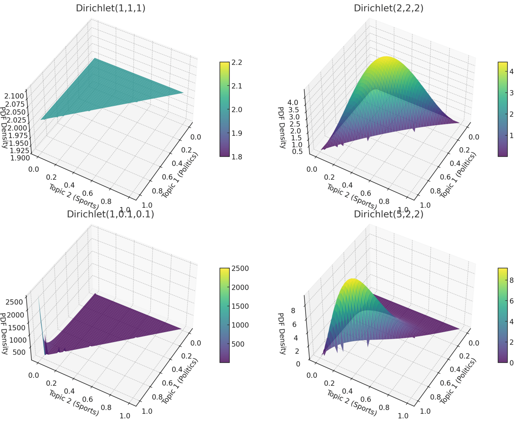
Details on the Dirichlet Distribution
K-dimensional Dirichlet distribution the probability density function (PDF) is:
P(θ∣α)=1B(α)∏i=1Kθiαi−1
where:
θ=(θ1,θ2,...,θK
\( \theta = (\theta_1, ..., \theta_K) \) represents a probability vector (e.g., a document's topic distribution).α=(α1,α2,...,αK
\( \alpha = (\alpha_1, ..., \alpha_K) \) is the Dirichlet parameter vector controlling the shape of the distribution.
-
B(α)\( B(a) \) is the normalizing constant (Beta function).
It ensures that the Dirichlet distribution integrates to 1.
$$ P(\theta \mid \alpha) = \frac{1}{B\alpha} \prod_{i=1}^{K} \theta_i^{\alpha_i-1} $$
The Dirichlet distribution for three topics (\(K=3\)) is:
\( P(\theta | \alpha) = \frac{1}{B(\alpha)} \theta_1^{\alpha_1 - 1} \theta_2^{\alpha_2 - 1} \theta_3^{\alpha_3 - 1} \)
\(\theta_1 + \theta_2 + \theta_3 = 1, \quad \text{with } \theta_i \geq 0 \)
where the Beta function \( B(\alpha) \) is:
\( B(\alpha) = \frac{\Gamma(\alpha_1) \Gamma(\alpha_2) \Gamma(\alpha_3)}{\Gamma(\alpha_1 + \alpha_2 + \alpha_3)} \)
and \( \Gamma(x) \) is the Gamma function:
\(\Gamma(x) = \int_0^\infty t^{x-1} e^{-t} \, dt\)
\( e \): Euler's number \( \approx 2.718 \)
\( t \): Integration Variable
\( B(\alpha) = \frac{\prod_{i=1}^{K} \Gamma(\alpha_i)}{\Gamma\left( \sum_{i=1}^{K} \alpha_i \right)} \)
where \( \Gamma(\cdot) \) is the Gamma function:
\( \Gamma(x) = \int_0^\infty t^{x-1} e^{-t} \, dt \)