Where do galaxies get their spin from?
They got it from their mama
A story of angular momentum,
tracer particles and data analysis
\(z ≥ 2\): some puzzle(s) of galactic disks
- Alignment at large scales
→ common origin of gal. spins
- Spin of DM halo ≠ spin of disk
→ diff. evol. of DM vs baryons
- Virial shock → should prevent coherent accretion
- Feedback → disk destruction?
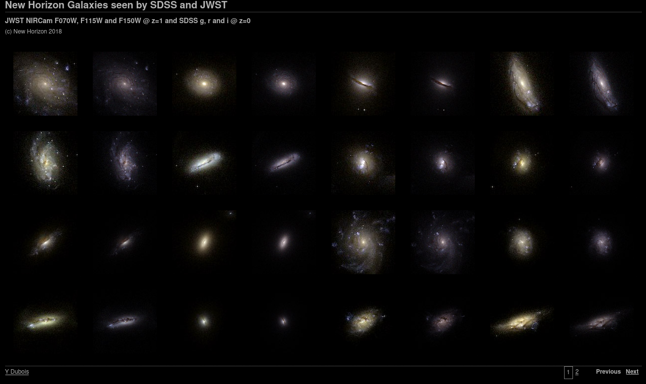

Filamentary accretion is responsible for most of the mass and angular momentum acquisition (at z>3 ; Kereš+05, Pichon+11, Tillson+12, …)
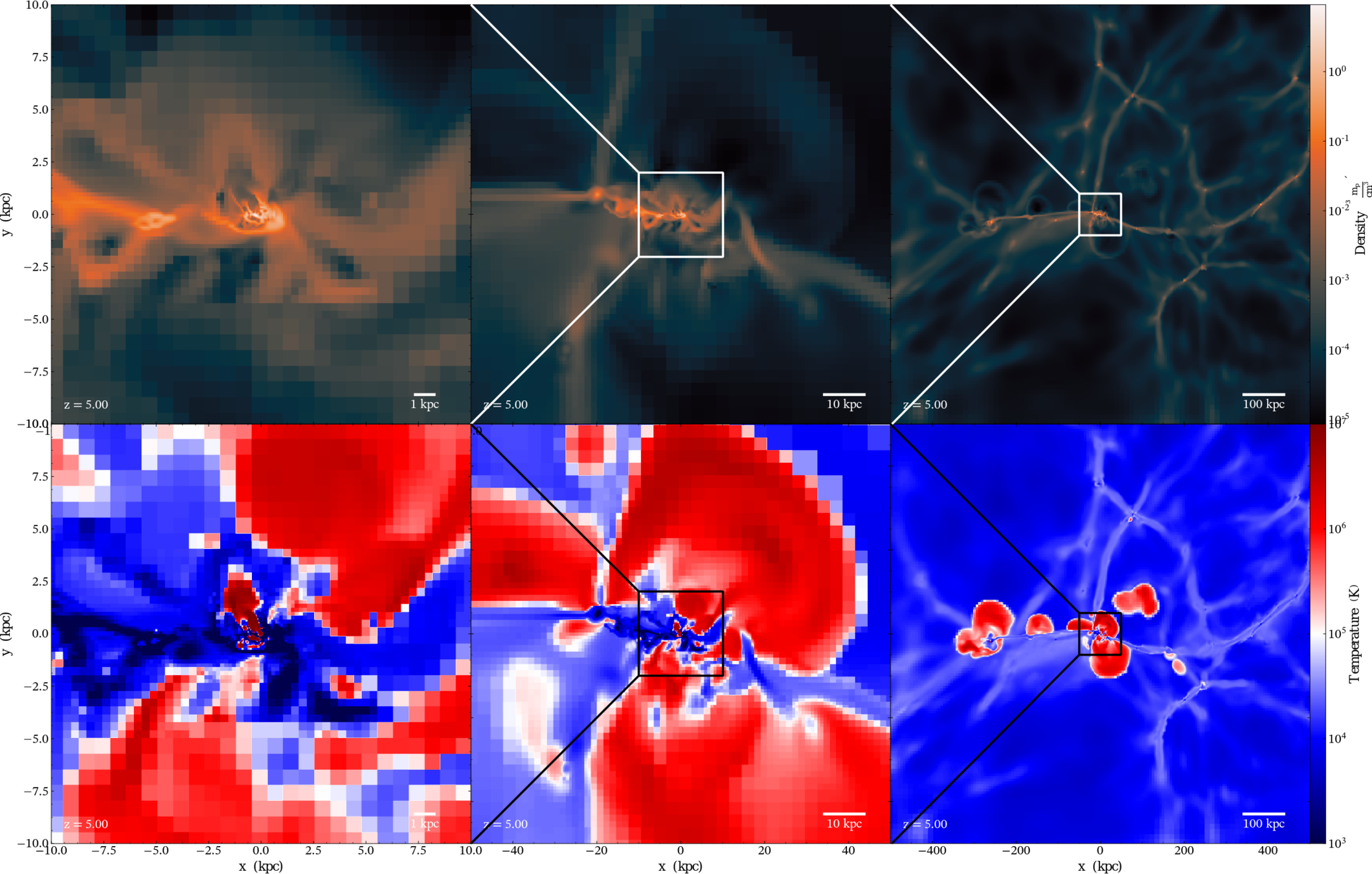
Filamentary accretion: natural "bridge" between large scale structures (cosmic web) and galaxy formation
What to do?
- Study AM kinematics,
- in accretion flows,
- both cold and hot,
- dynamics: compute torques,
- here, pressure & gravitational torques.
- easy, \(\sum m \mathbf{r}\times \mathbf{v}\)
- Lagrangian trajectories
- temperature along Lagrangian traj.
- easy, right? \(\sum \mathbf{r}\times \mathbf{f}\)
- \(\nabla P, \nabla \phi\)
(grav. accel. provided by simulation)
Tracer particles
Eulerian method
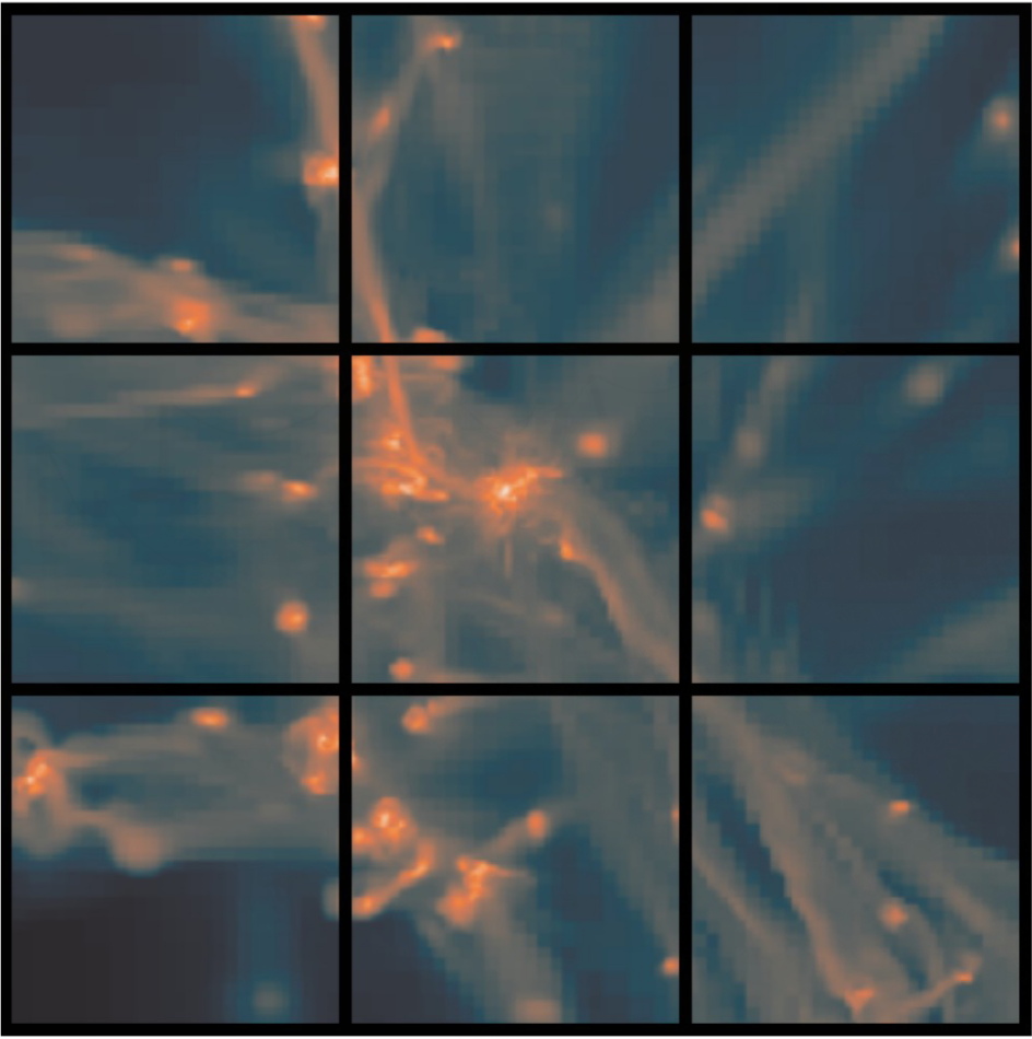
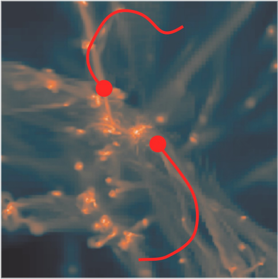
Lagrangian history
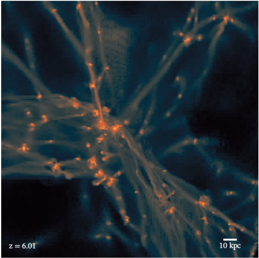
Tracer particles!

Eulerian method
How to access Lagrangian history in Eulerian simulation?

?

Lagrangian history
Tracer particles!
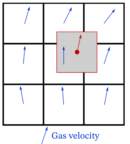
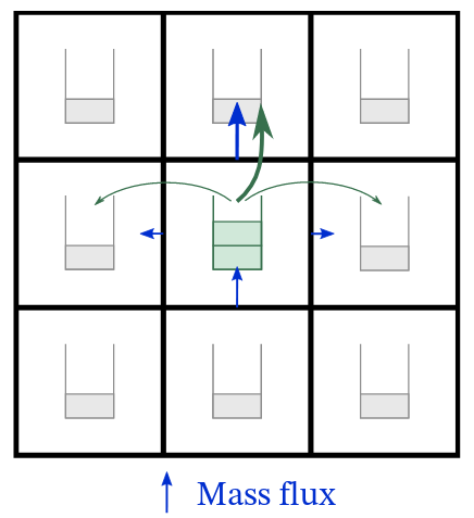
\(v\)-based tracers
Using linear interpolation of velocity
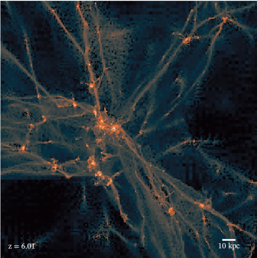

MC-based tracers
\[p_{i,j} \propto \mathrm{flux}(i\rightarrow j)\]
Bonus: also work for SF, feedback, …

Eulerian method
How to access Lagrangian history in Eulerian simulation?

\(v\)-based tracers
Using linear interpolation of velocity


MC-based tracers
\[p_{i,j} \propto \mathrm{flux}(i\rightarrow j)\]
Bonus: also work for SF, feedback, …


-
-
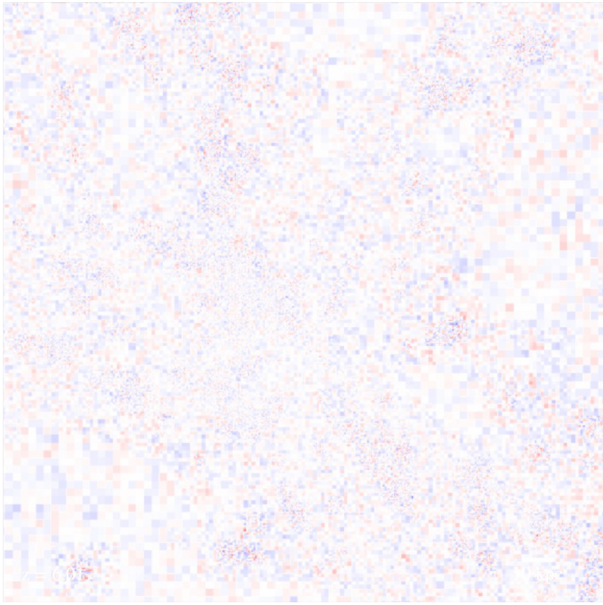
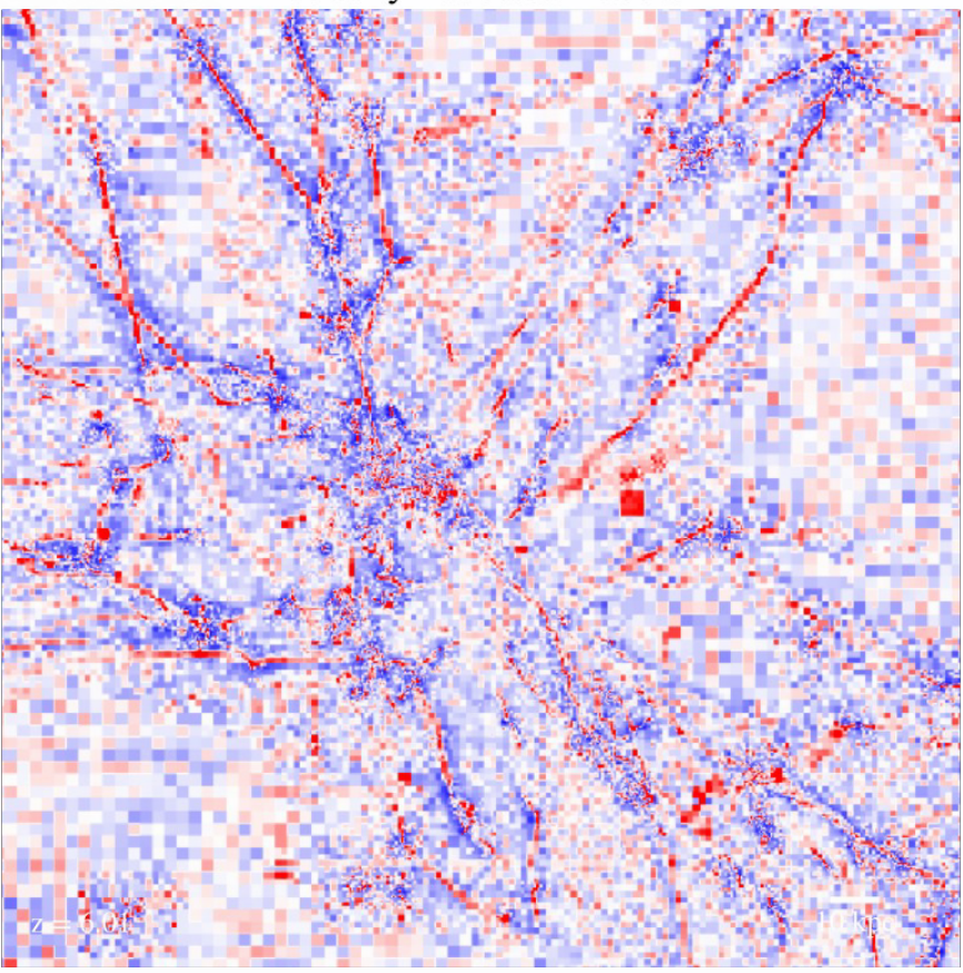
=
=
Reference
Reference
Difference
Difference
\(v\)-based tracers
Using linear interpolation of velocity


MC-based tracers
\[p_{i,j} \propto \mathrm{flux}(i\rightarrow j)\]
Bonus: also work for SF, feedback, …

What to do?
- Study AM kinematics,
- in accretion flows,
- both cold and hot,
- dynamics: compute torques,
- here, pressure & gravitational torques.
✅ easy, \(\sum m \mathbf{r}\times \mathbf{v}\)
❔ Lagrangian trajectories
❔ temperature along Lagrangian traj.
❔ easy, right? \(\sum \mathbf{r}\times \mathbf{f}\)
❔ \(\nabla P, \nabla \phi\)
(grav. accel. provided by simulation)
What to do?
- Study AM kinematics,
- in accretion flows,
- both cold and hot,
- dynamics: compute torques,
- here, pressure & gravitational torques.
✅ easy, \(\sum m \mathbf{r}\times \mathbf{v}\)
✅ Lagrangian trajectories
❔ temperature along Lagrangian traj.
❔ easy, right? \(\sum \mathbf{r}\times \mathbf{f}\)
❔ \(\nabla P, \nabla \phi\)
(grav. accel. provided by simulation)
Grid data
Particle data


Easy!
Use cic/nearest interpolation
yt.add_deposited_particle_fields(
    ("tracer", "particle_mass"),
    method="cic"
)
p = yt.ProjectionPlot(
  ds,
  ("deposit", "tracer_cic_mass")
)
Grid data
Particle data


(Now it is) easy!
Use "mesh deposition"
ds.add_mesh_sampling_particle_field(
  ("gas", "density"),
  "tracer"
)
ds.r["tracer", "cell_gas_density"]
# Took 1.4s for 1 090 895 particles!

p = yt.ParticleProjectionPlot(
  ds,
  ("tracer", "cell_gas_density")
)
pos = ds.r["tracer", "particle_position"][:1000]
new_data = ds.arr([
  ds.r[p]["density"]
  for p in pos
])

# Argh! Took 3.5s for 1 000 particles!
# ETA: 1hr for all particles
Easy?
ds.add_mesh_sampling_particle_field(
  ("gas", "density"),
  "tracer"
)

# Precompute cell index
ds.r["tracer", "cell_index"]        # 1.3s

# Fast access!
ds.r["tracer", "cell_gas_density"]  # 300ms
What to do?
- Study AM kinematics,
- in accretion flows,
- both cold and hot,
- dynamics: compute torques,
- here, pressure & gravitational torques.
✅ easy, \(\sum m \mathbf{r}\times \mathbf{v}\)
✅ Lagrangian trajectories
❔ temperature along Lagrangian traj.
❔ easy, right? \(\sum \mathbf{r}\times \mathbf{f}\)
❔ \(\nabla P, \nabla \phi\)
(grav. accel. provided by simulation)
What to do?
- Study AM kinematics,
- in accretion flows,
- both cold and hot,
- dynamics: compute torques,
- here, pressure & gravitational torques.
✅ easy, \(\sum m \mathbf{r}\times \mathbf{v}\)
✅ Lagrangian trajectories
✅ temperature along Lagrangian traj.
✅ easy, right? \(\sum \mathbf{r}\times \mathbf{f}\)
❔ \(\nabla P, \nabla \phi\)
(grav. accel. provided by simulation)
$$ \nabla P =\frac{P_{i+1} - 2P_i + P_{i-1}}{2} $$
Gradient needs (at least) 3 cells in each direction,
but octrees only have 2!
Background: https://www.youtube.com/watch?v=Mf7P5hqD0eY
only 2 cells
$$ \nabla P =\frac{P_{i+1} - 2P_i + P_{i-1}}{2} $$
Gradient needs (at least) 3 cells in each direction,
but octrees only have 2!
Background: https://www.youtube.com/watch?v=Mf7P5hqD0eY
only 2 cells
Let us "extend" our octs with "ghost zones"


$$ \nabla P =\frac{P_{i+1} - 2P_i + P_{i-1}}{2} $$
Gradient needs (at least) 3 cells in each direction,
but octrees only have 2!
Background: https://www.youtube.com/watch?v=Mf7P5hqD0eY
now 4 cells wide!
Let us "extend" our octs with "ghost zones"


\(P_{i+1}\)
\(P_{i-1}\)
\(P_{i}\)
$$ \nabla P =\frac{P_{i+1} - 2P_i + P_{i-1}}{2} $$
Gradient needs (at least) 3 cells in each direction,
but octrees only have 2!
Background: https://www.youtube.com/watch?v=Mf7P5hqD0eY
now 4 cells wide!
Let us "extend" our octs with "ghost zones"


\(P_{i+1}\)
\(P_{i-1}\)
\(P_{i}\)
I am only showing 6 out of 56 ghost cells for clarity.
But trust me they are here.
You can also use more than 2-cells (for higher order derivatives).
What to do?
- Study AM kinematics,
- in accretion flows,
- both cold and hot,
- dynamics: compute torques,
- here, pressure & gravitational torques.
✅ easy, \(\sum m \mathbf{r}\times \mathbf{v}\)
✅ Lagrangian trajectories
✅ temperature along Lagrangian traj.
✅ easy, right? \(\sum \mathbf{r}\times \mathbf{f}\)
❔ \(\nabla P, \nabla \phi\)
(grav. accel. provided by simulation)
What to do?
- Study AM kinematics,
- in accretion flows,
- both cold and hot,
- dynamics: compute torques,
- here, pressure & gravitational torques.
✅ easy, \(\sum m \mathbf{r}\times \mathbf{v}\)
✅ Lagrangian trajectories
✅ temperature along Lagrangian traj.
✅ easy, right? \(\sum \mathbf{r}\times \mathbf{f}\)
✅ \(\nabla P, \nabla \phi\)
(grav. accel. provided by simulation)
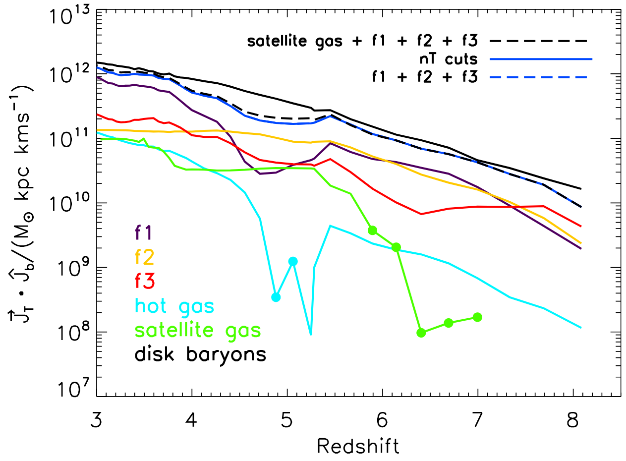
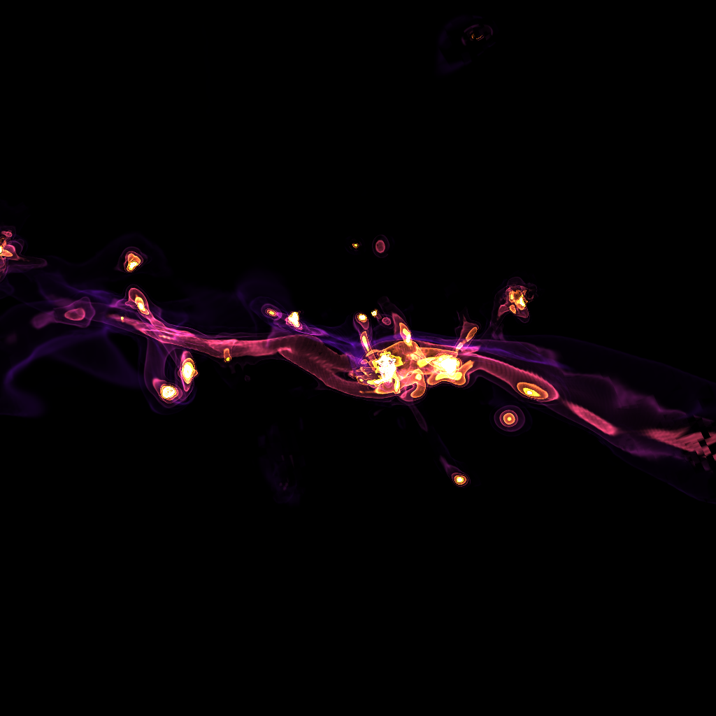
Inspecting Kinematics
Plot of \( \frac{1}{\Delta r}\int_{r}^{r+\Delta r} \mathrm{d}r\,\mathbf{r} \times \mathbf{v}\)
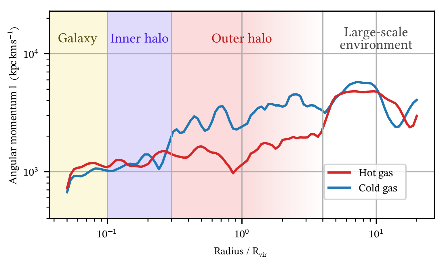
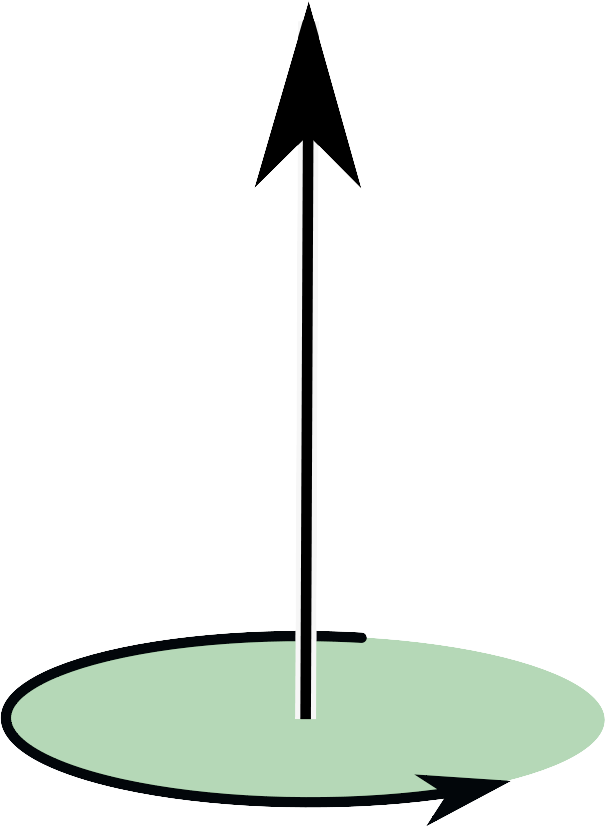
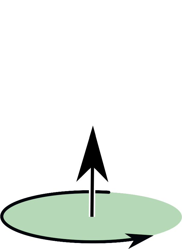
Large scale
Galaxy
Direction of accretion
drop by \(\times 5\)
So the AM drops by \(\times 5\)
(in one free-fall time)
(Local) dynamics
The AM dynamics is given by

\(\displaystyle \phantom{\frac{\mathrm{d} \mathbf{l}}{\mathrm{d} t}} + \text{gravitational torques} \)
\( \displaystyle \frac{\mathrm{d} \mathbf{l}}{\mathrm{d} t} = \textcolor{darksalmon}{\text{pressure torque}} \)
\(\displaystyle \phantom{\frac{\mathrm{d} \mathbf{l}}{\mathrm{d} t} + } \underbrace{\phantom{\text{gravitational torques}}}_{\text{\textcolor{darkgray}{DM} + \textcolor{orange}{Star} + \textcolor{deepskyblue}{Gas}}} \)
Pressure dominates the ⊥ acceleration in CGM…
locally!
Mean of ⊥ force magnitude

(Global) dynamics
Compute global torque in shell


Dynamics
Locally: pressure dominated...
esp. in the hot phase


... but globally: (DM) gravity dominated
esp. in the cold phase
What is happening?


Spatial-coherence of torques
Compute sum-of-norm vs norm-of-sum
$$ \dfrac{\left\| \sum_\text{neigh}\tau\right\|}{ \sum_\text{neigh}\left\| \tau\right\|} $$
Pressure: \(\lambda_\mathrm{fluct.}\) is small


Gravity
Pressure


Spatial-coherence of torques
Compute sum-of-norm vs norm-of-sum
$$ \dfrac{\left\| \sum_\text{neigh}\tau\right\|}{ \sum_\text{neigh}\left\| \tau\right\|} $$

Pressure: \(\lambda_\mathrm{fluct.}\) is small
Conclusions
Conclusions
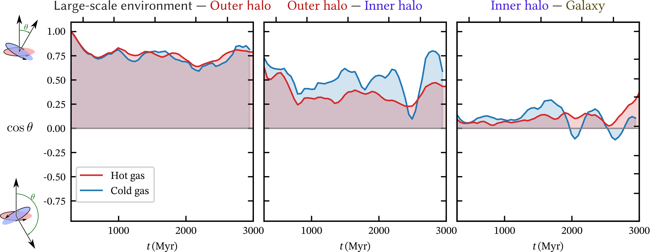
Kinematics:
- AM transported through CGM
- orientation mostly retained down to outer disk

Dynamics:
- pressure locally dominant (esp. in hot)
- gravity globally dominant (esp. in cold)
- torques have spatial & time variations ⇒ need careful treatment


Conclusions
Many cool features brought together!
- [RAMSES] Lagrangian tracer
- [yt] mesh sampling
-
[yt] "ghost zones" for octrees
- enable gradient computation
- but also vertex centred!
Cold gas selection
( \( \forall t, T(t)\leq 10⁵\ \mathrm{K} \) and
\( 0.3 R_\mathrm{vir} \leq r(t) \leq 2 R_\mathrm{vir} \))
or
$$ r < 0.3 R_\mathrm{vir} \text{ or } r > 2R_\mathrm{vir} $$
Hot gas selection
$$ \exists t, T(t)> 10⁵\ \mathrm{K} \\ 0.3 R_\mathrm{vir} \leq r(t)\leq 2 R_\mathrm{vir} $$
⇒ Defined with Lagrangian history
+ removing accretion from satellites

Kinematics
Cold gas: well aligned down to inner halo
Hot gas: aligned down to inner halo


Simulation setup
- suite of zoom-in simulations (~6), RAMSES (Teyssier 2002)
- Δx = 35pc, Mstar = 1.1 10⁴ M☉ Mhalo=10¹² M☉
- Turbulent star formation (Kimm+17, Trebitsch+17)
- Mechanical feedback (Kimm+15)
- AGN formation with spin-regulated efficiency (Dubois+12,+14)
- 30,000,000 tracer particles (~10/cell, 0.5/star, Cadiou+19)

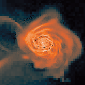
Gas density
Gas tracer density

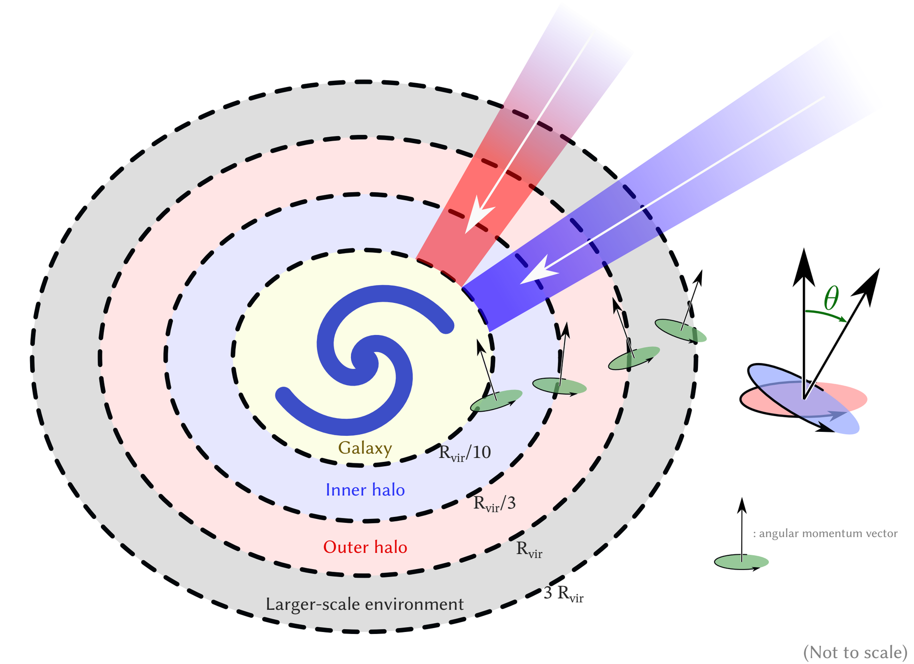
3. Contribution to disk formation
1. AM acquisition at large scale
2. Transport along cold flows


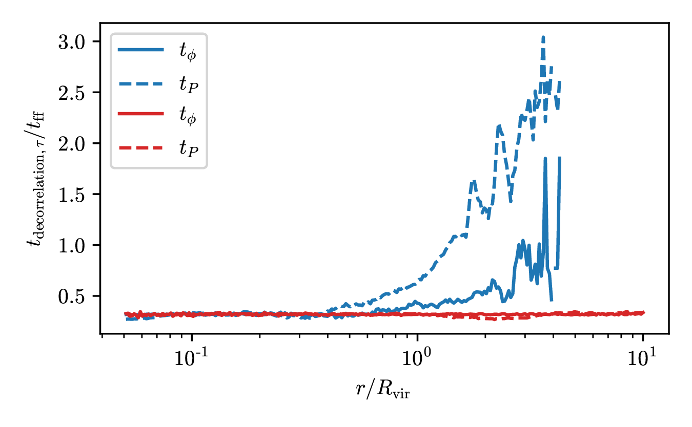
Time-coherence of torques
Compute \(t_\mathrm{decorr.}\) using Lagrangian history such that
$$ \vec{\tau}(t_\mathrm{decorr.}) \perp \vec{\tau}(0) \color{gray}\qquad\text{ (i.e. } \vec{\tau}(t_\mathrm{decorr.}) \cdot \vec{\tau}(0) = 0)$$
A/ Longer coherence in cold phase (esp. pressure)
Slow decorrelation
Fast decorrelation


Density \(\rho\)

\(v\) tracers
MC tracers
Difference \(\Delta \rho / \rho\)
Applications
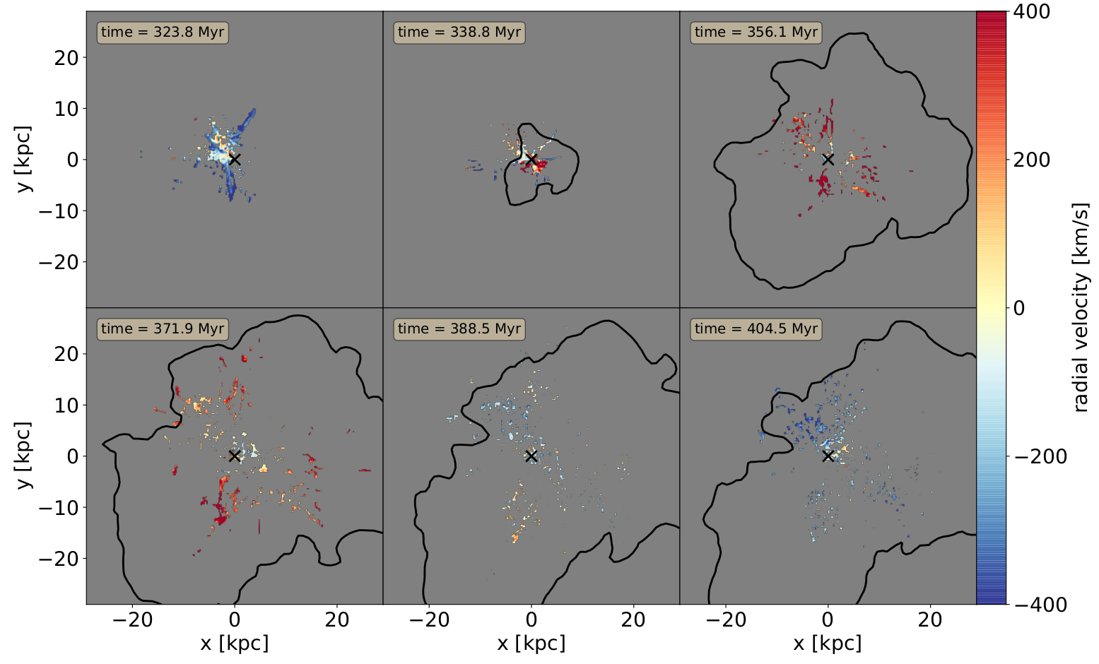
Formation & destruction of filamentary structures in Perseus-like cluster
Tracer: history of each clump
Beckmann+19
Applications
Study of gas in & out — origin of Ly\(\alpha\) emitting gas
Mitchell+20
