Angular momentum evolution can be predicted from cosmological initial conditions

With A. Pontzen & H. V. Peiris — arXiv:2012.02201

The origin of angular momentum

Galaxies → origin of rotational support?
Physics → origin of vector quantity irrotational field?
Cosmology → origin of spin alignment signal?

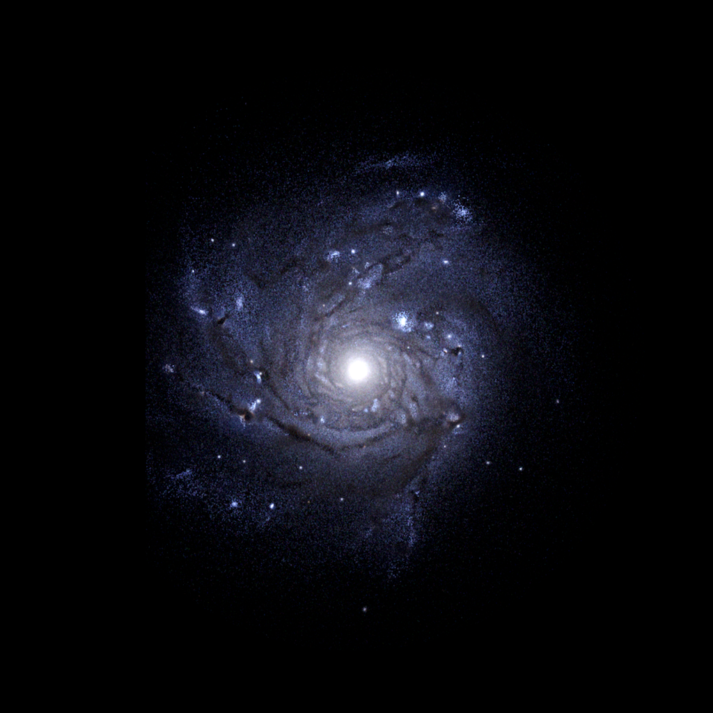
New-Horizon simulation — Dubois+20

Tempel+13

Focus on closed systems: Lagrangian patch

Predict one value for $ \vec{L} $

Focus on open systems: dark matter haloes

Predict $ p(\vec{L}) $

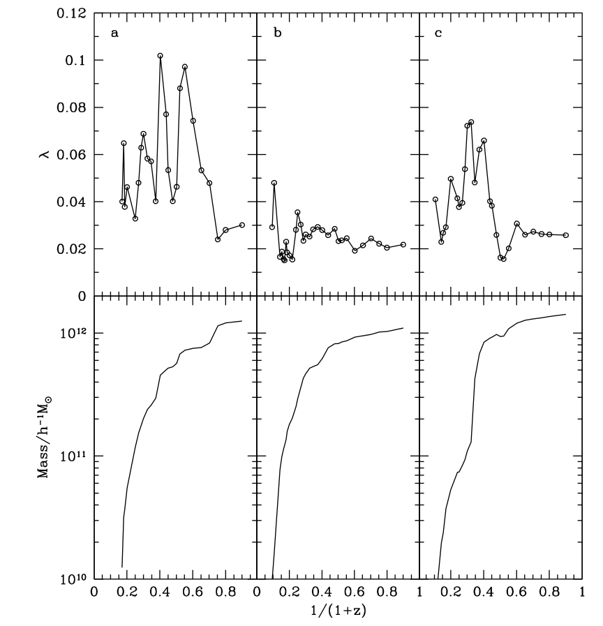
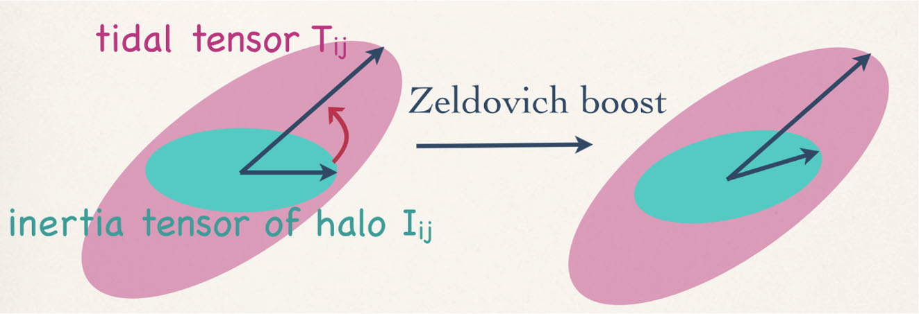
Tidal Torque Theory

& semi-Analytical Models

$$ \vec{L} = a^2 \dot{D} \vec{L}_0 $$

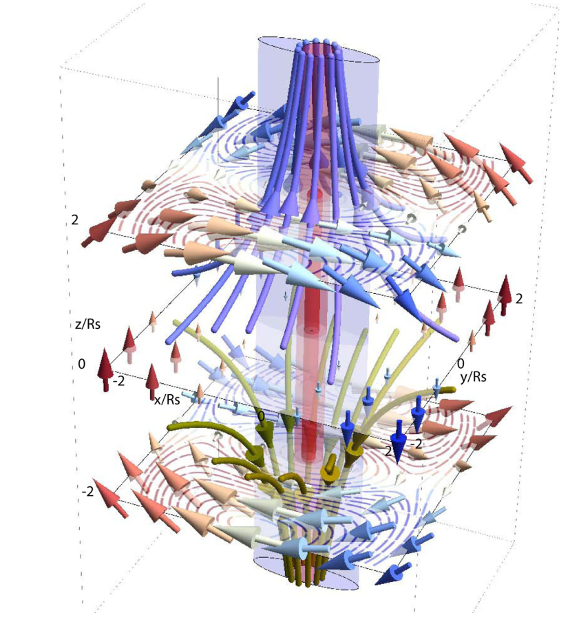
White 84, Codis+15

Vitvitska+02

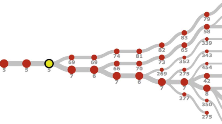
AM can be predicted

AM is stochastic/chaotic

TTT

Focus on closed systems: Lagrangian patch

Predict one value for $ \vec{L} $

sAMs

Focus on open systems: dark matter haloes

Predict $ p(\vec{L}) $

TTT & semi-analytical models

AM can be predicted from the initial conditions

AM is stochastic/chaotic

Is AM chaotic or not?

Not chaotic if for a given region,

$$ \vec{L}(t) = {\color{red}f(t)} \times \color{blue}\vec{L}_0,\phantom{(1+\epsilon),} $$

with $\color{red} f$ indep. of $\color{blue}\vec{L}_0$.

Is AM chaotic or not?

Not chaotic if for a given region,

$$ \vec{L}(t) = {\color{red}f(t)} \times \color{blue}\vec{L}_0\phantom{,}{(1+\epsilon)}, $$

with $\color{red} f$ indep. of $\color{blue}\vec{L}_0$.

Is AM chaotic or not?

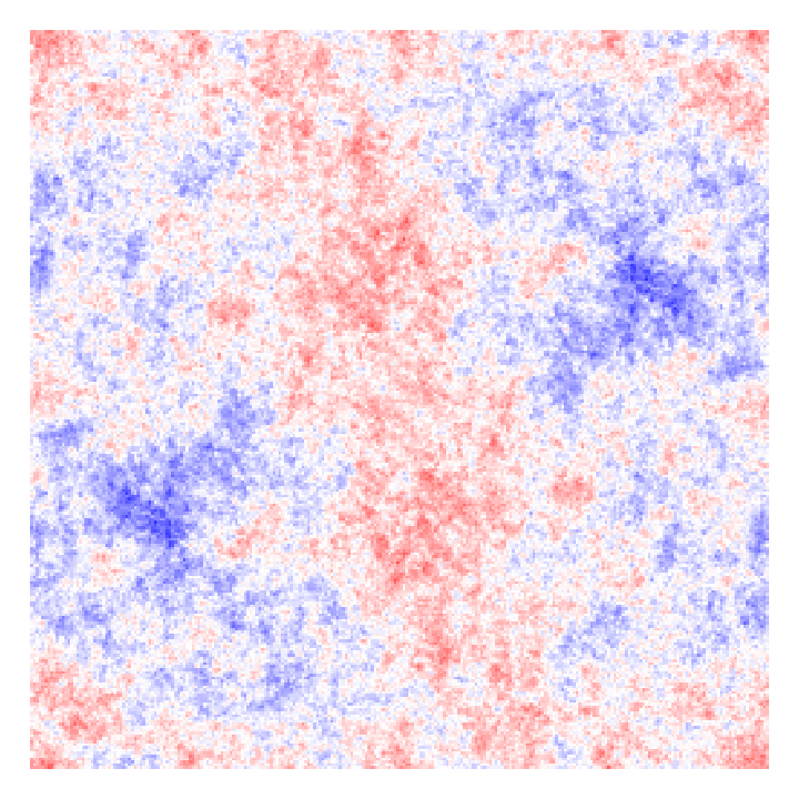
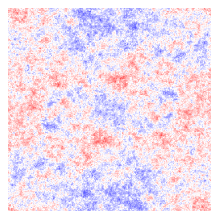
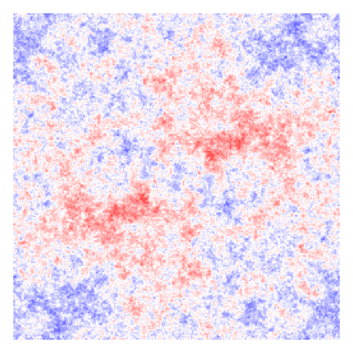
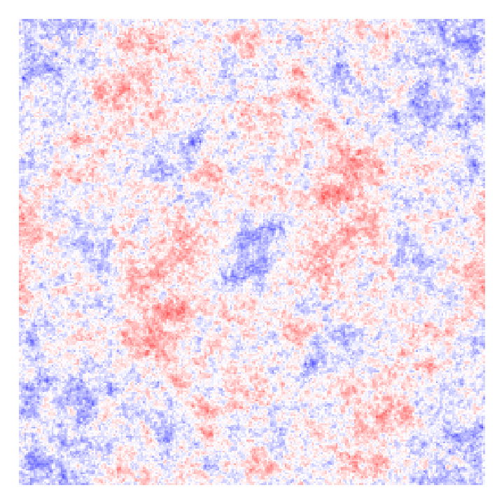
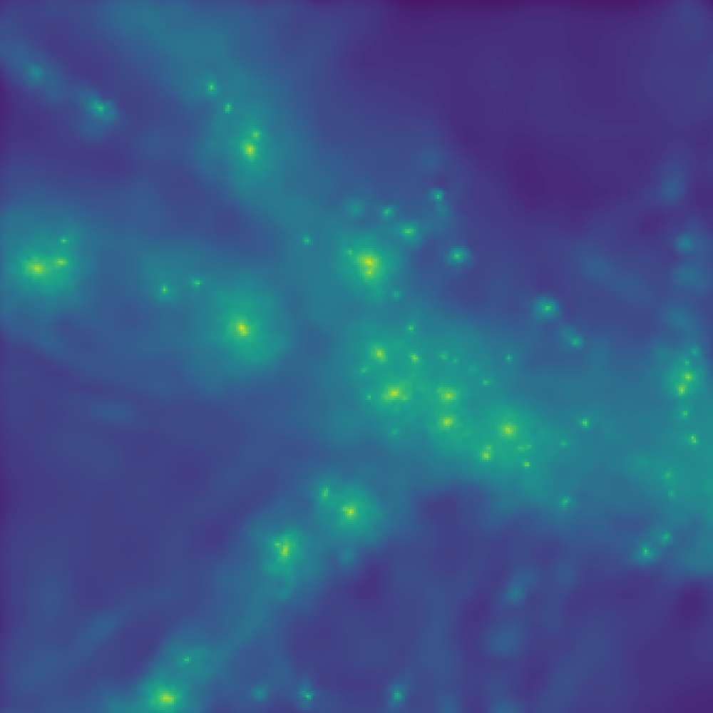
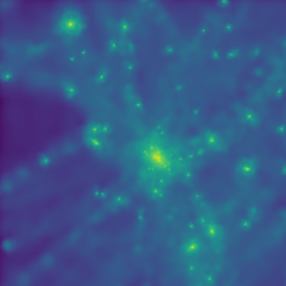
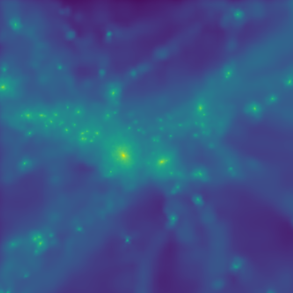
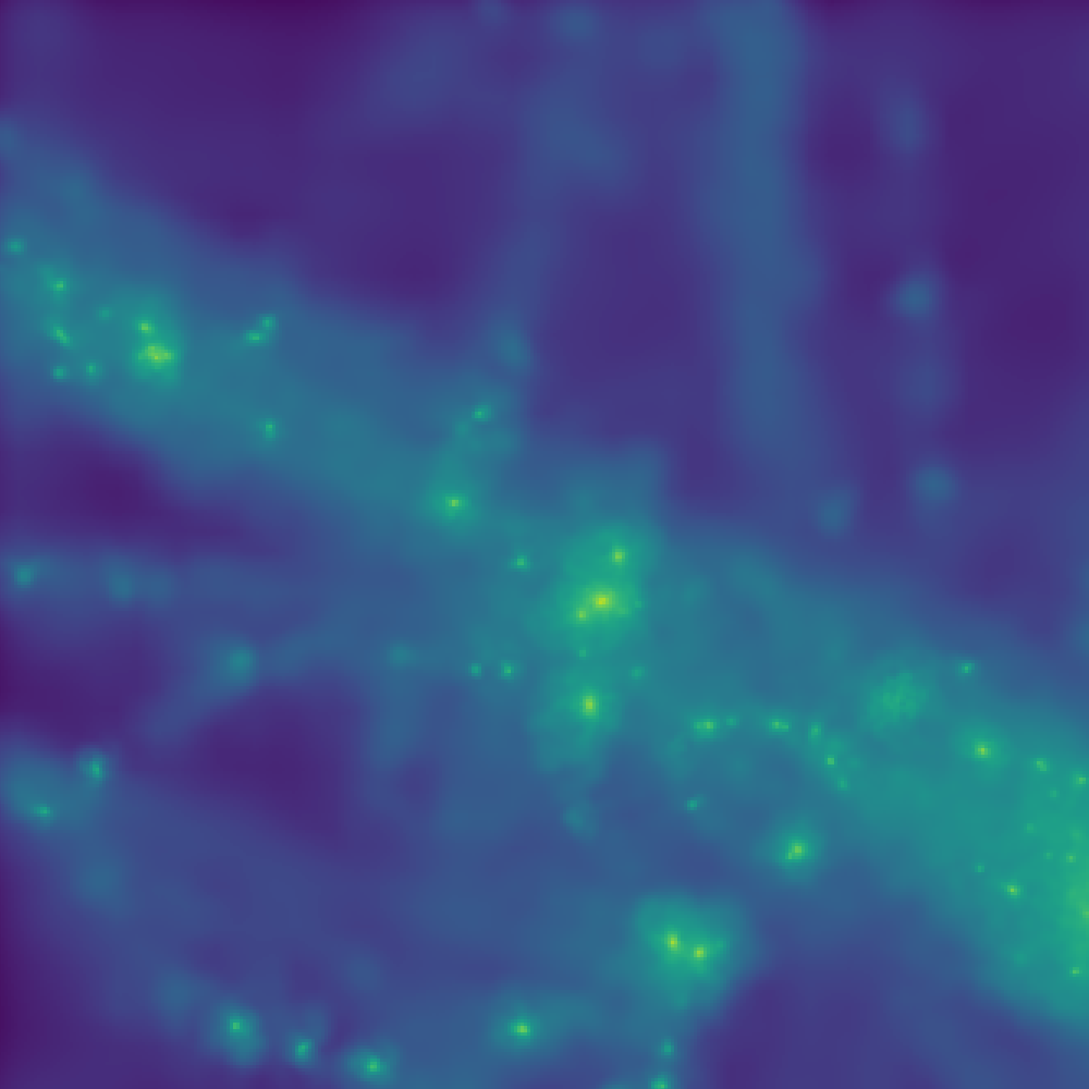
How to change $\color{blue}\vec{L}_0$ all other things being equal?

$\Lambda$CDM gives you $\neq\color{blue} \vec{L}_0$ … all other things different.

*Only an illustration, ICs do not correspond to the halos below.

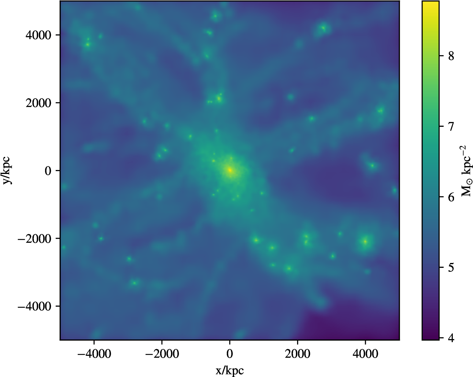
$N$-body numerical integration

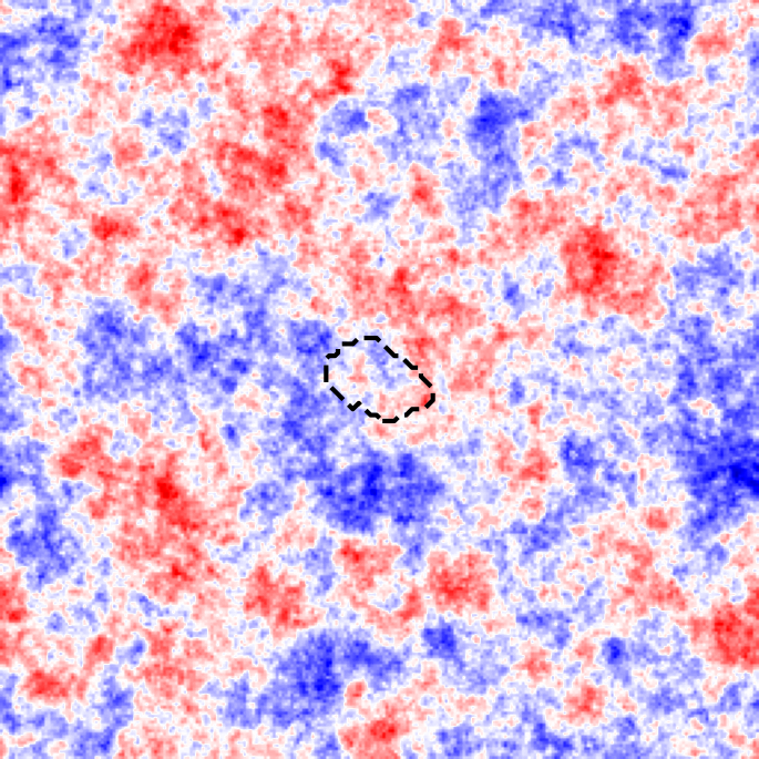
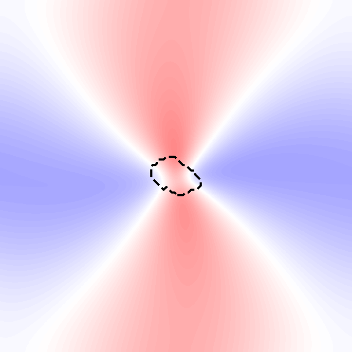
Original $\vec{L}_0$

Genetic modif.

$N$-body numerical integration

Contrast x50

Roth+15, Stopyra+20

Can compute

$$ P\big(\delta \big| \delta(x) = v\big) $$

$$ P\Big(\delta \Big| \sum_i \alpha_i \delta_i = v\Big) $$

$$ P\Big(\delta \Big| L_x = v \Big) $$

+ minimization of $\Delta \chi^2$
⇒ unique solution
= "genetically modified density field"

Original $\vec{L}_0$

Genetic modif.

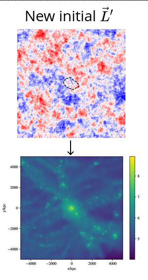
New initial $\vec{L}_0'$

$N$-body numerical integration

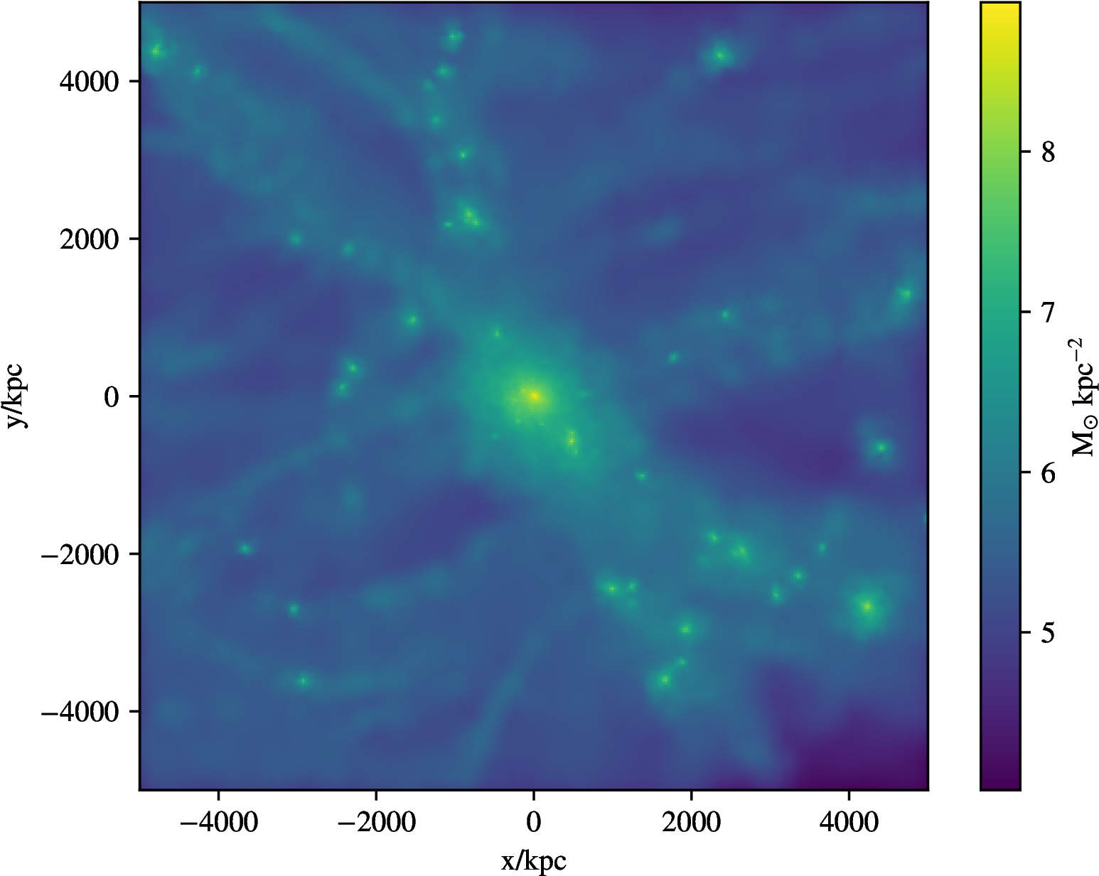
$N$-body numerical integration

Same region & environment

Different $\color{blue} \vec{L}_0$

Contrast x50

Roth+15, Stopyra+20

Original $\vec{L}_0$

New initial $\vec{L}_0'$

Original $\vec{L}$

New initial $\vec{L}'$

We can predict/control AM down to $z = 0$.*

How does it compare to predictions from linear theory?

*AM of regions, not halos

Prediction from linear theory:

$$ \vec{L}_\mathrm{pred.} = {\color{blue}\underbrace{\quad a^2\dot{D} \quad}_{\color{blue}\mathrm{time}}} \times {\color{red}\underbrace{\quad\vec{L}_0\quad}_{\mathrm{space}}}.$$

Simulations with genetically modified initial conditions

$$ \vec{L}_\mathrm{pred.} = {\color{blue}\underbrace{\quad f(t) \quad}_{\color{blue}\mathrm{time}}} \times {\color{red}\underbrace{\quad\vec{L}_0\quad}_{\mathrm{space}}},$$
where $\color{blue}f(t)$ is the measured growth rate of a given region in the ref. simu.

Comparison with tidal torque theory

Prediction from linear theory:

$$ \vec{L}_\mathrm{pred.} = {\color{blue}\underbrace{\quad a^2\dot{D} \quad}_{\color{blue}\mathrm{time}}} \times {\color{red}\underbrace{\quad\vec{L}_0\quad}_{\mathrm{space}}}.$$

Simulations with genetically modified initial conditions

$$ \vec{L}_\mathrm{pred.} = {\color{blue}\underbrace{\quad f(t) \quad}_{\color{blue}\mathrm{time}}} \times {\color{red}\underbrace{\quad\vec{L}_0\quad}_{\mathrm{space}}},$$where $\color{blue}f(t)$ is the measured growth rate of a given region in the ref. simu.

Comparison with tidal torque theory

Median of deviations

Prediction from linear theory:

$$ \vec{L}_\mathrm{pred.} = {\color{blue}\underbrace{\quad a^2\dot{D} \quad}_{\color{blue}\mathrm{time}}} \times {\color{red}\underbrace{\quad\vec{L}_0\quad}_{\mathrm{space}}}.$$

Simulations with genetically modified initial conditions

$$ \vec{L}_\mathrm{pred.} = {\color{blue}\underbrace{\quad f(t) \quad}_{\color{blue}\mathrm{time}}} \times {\color{red}\underbrace{\quad\vec{L}_0\quad}_{\mathrm{space}}},$$where $\color{blue}f(t)$ is the measured growth rate of a given region in the ref. simu.

Comparison with tidal torque theory

Median of deviations

Scatter of deviations

Prediction from linear theory:

$$ \vec{L}_\mathrm{pred.} = {\color{blue}\underbrace{\quad a^2\dot{D} \quad}_{\color{blue}\mathrm{time}}} \times {\color{red}\underbrace{\quad\vec{L}_0\quad}_{\mathrm{space}}}.$$

Simulations with genetically modified initial conditions

$$ \vec{L}_\mathrm{pred.} = {\color{blue}\underbrace{\quad f(t) \quad}_{\color{blue}\mathrm{time}}} \times {\color{red}\underbrace{\quad\vec{L}_0\quad}_{\mathrm{space}}},$$where $\color{blue}f(t)$ is the measured growth rate of a given region in the ref. simu.

Comparison with tidal torque theory

Median of deviations

Scatter of deviations

Much more accurate pred. than linear theory
Departure happen at later time
The smaller the modif., the smaller the scatter
⇒ linear response

Conclusions

Explored how $\vec{L}$ of given fixed regions changes with changed $\color{blue}\vec{L}_0$

angular momentum can be predicted accurately from initial conditions (not chaotic)
possible to improve linear theory by predicting growth rate $\color{red} f(t)$
apparent stochasticity of AM of halos ⇒ result of particle membership

Read more in Cadiou, Pontzen & Peiris arXiv:2012.02201.

Conclusions

What's next?

apply to baryons instead of DM only?
extend analysis to halos?
predict $\color{red}f(t)$ rather than measure it?

Read more in Cadiou, Pontzen & Peiris arXiv:2012.02201.

Explored how $\vec{L}$ of given fixed regions changes with changed $\color{blue}\vec{L}_0$

angular momentum can be predicted accurately from initial conditions (not chaotic)
possible to improve linear theory by predicting growth rate $\color{red} f(t)$
apparent stochasticity of AM of halos ⇒ result of particle membership

AM genetic modifications

Initial $\vec{L}$ given in initial conditions by

$$ L_{z,0} \propto \sum_{i,j,k}\left[ (q_{x}^{ijk} - \bar{q}_x) \nabla_y\phi^{ijk} - (q_{y}^{ijk} - \bar{q}_y) \nabla_x\phi^{ijk}\right]. $$

Genetic modifications: find $\vec{u}$ such that

$$ \vec{u} \cdot \vec{\delta} = \vec{L}_0,$$

with $\vec{\delta} = \{\delta^{i_0j_0k_0}, \dots, \delta^{i_nj_nk_n}\} $ and solve for

$$ \vec{u}\cdot \vec{\delta}' = \vec{L}_0'$$

with minimal change.