Corentin Cadiou\({}^1\) (cadiou@iap.fr)

Lead developers: Maxime Delorme (CEA), Arnaud Durocher (CEA)

Scientific collaborators:
Dominique Aubert (ObAS), Olivier Marchal (ObAS), San Han (IAP), Guillaume Tcherniatinsky (IAP), Harley Katz (U. Chicago), …

\({}^1\)Institut d’Astrophysique de Paris, CNRS, France

Dyablo:
A New General-Purpose
GPU-Accelerated
Hydrodynamical Code for Astrophysics

Credits: M. Delorme

Data: Top-500

Manage grid, simple computation

Computation-heavy
(hydro, gravity, …)

CPU

GPU

[…]

wasted
time

Typical approach: offloading

Dyablo's approach:

Amdahl's law: latency kills gains of parallelisation

Manage grid, simple computation

Computation-heavy
(hydro, gravity, …)

CPU

GPU
(or CPUs)

[…]

Typical approach: offloading

Dyablo's approach: “true” GPU computing, CPU as a puppeteer

Manage grid, simple computation

Computation-heavy
(hydro, gravity, …)

[…]

Typical approach: offloading

Dyablo's approach: “true” GPU computing, CPU as a puppeteer

1. Separation of concerns

Physicists: write subgrid models

Computer scientists:
optimize the code

2. Abstraction

Physics: independent of data layout, parallelization, ...

Code should provide high-level APIs

3. Modularity

Implementations & models should be interchangeable depending on needs

CPU

GPU
(or CPUs)

Dyablo: Overall design

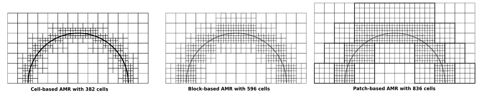
Cell or block-based

Adaptive Mesh Refinement

Collection of \(N\times M\times L\) blocks

Traditional oct-based AMR

Dyablo: Overall design

[...]

// Memory abstracted
Kokkos::View<double**> U(Ncell, Nfields);

// Parallelism abstracted
Kokkos::parallel_for(Ncell, KOKKOS_LAMBDA(size_t iCell) {
   U(iCell, IRho) += ...
});

[...]

Single node / GPU

Dyablo: Overall design

[...]

// Memory abstracted
Kokkos::View<double**> U(Ncell, Nfields);

// Parallelism abstracted
Kokkos::parallel_for(Ncell, KOKKOS_LAMBDA(size_t iCell) {
   U(iCell, IRho) += ...
});

[...]

[...]

// Memory abstracted
Kokkos::View<double**> U(Ncell, Nfields);

// Parallelism abstracted
Kokkos::parallel_for(Ncell, KOKKOS_LAMBDA(size_t iCell) {
   U(iCell, IRho) += ...
});

[...]

[...]

// Memory abstracted
Kokkos::View<double**> U(Ncell, Nfields);

// Parallelism abstracted
Kokkos::parallel_for(Ncell, KOKKOS_LAMBDA(size_t iCell) {
   U(iCell, IRho) += ...
});

[...]

[...]

// Memory abstracted
Kokkos::View<double**> U(Ncell, Nfields);

// Parallelism abstracted
Kokkos::parallel_for(Ncell, KOKKOS_LAMBDA(size_t iCell) {
   U(iCell, IRho) += ...
});

[...]

[...]

// Memory abstracted
Kokkos::View<double**> U(Ncell, Nfields);

// Parallelism abstracted
Kokkos::parallel_for(Ncell, KOKKOS_LAMBDA(size_t iCell) {
   U(iCell, IRho) += ...
});

[...]

Dyablo: Implemented physics

Block-based adaptive mesh-refinement,
Hydrodynamics / MHD / radiative transfer
(Self-)Gravity
Particles,
Diffusion terms: thermal conduction, viscosity,
Cosmology: Comoving coordinates,
— Ongoing —
Star formation and feedback,
(Non-equilibrium) thermochemistry,
Cosmic rays, ...

Solar convection (Delorme)

Zeldovich pancake (Aubert & Marchal)

Halo mass function (Aubert & Marchal)

Thermochem. (Cadiou & Katz)

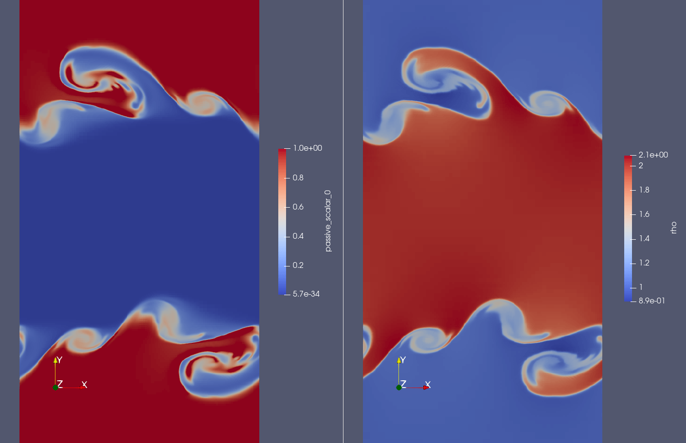
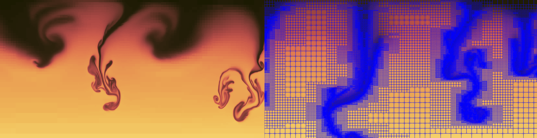
KH instability (Delorme)

Dyablo: how does it scale?

— weak scaling: solar convection

Image credits: Maxime Delorme

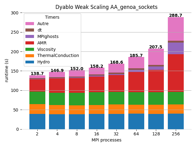
Ad Astra CPU (2 x AMD Epyc Genoa 96 cores )

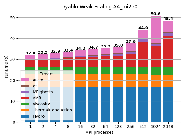
Ad Astra GPU (4 AMD MI250 x2 GCD )

Note: some updates in the code between left & right, raw perfs cannot be compared directly

Hydro only: \(\sim 200\,\mathrm{Mcell/s}\)

AthenaK \(\sim1000\,\mathrm{Mcell/s}\), Stone+24
Cholla-MHD \(\sim 200\, \mathrm{Mcell/s}\), Caddy+24,
AREPO-RT \(\sim 1\,\mathrm{Mcell/s}\), Zier+24

Shamrock \(\sim 10\,\mathrm{Mcell/s}\), David-Cléris+25

24,576 cores

Dyablo:
A New General-Purpose
GPU-Accelerated
Hydrodynamical Code for Astrophysics

Physics: hydrodynamics, MHD, RT, gravity, cosmology, ...

Efficient scaling up to 10,000+ CPUs, 1000+ GPUs

Modular and future-proof code

Credits: M. Delorme

Dyablo-HPC/Dyablo

Corentin Cadiou (cadiou@iap.fr)

3. Modularity

Implementations & models should be interchangeable depending on needs

1. Separation of concerns

Physicists: write subgrid models

Computer scientists:
optimize the code

2. Abstraction

Physics: independent of data layout, parallelization, ...

Code should provide high-level APIs

Dyablo: development methods

Dyablo: how does it scale?

— strong scaling

Image credits: Arnaud Durocher

Scaling test with replicated explosions (one per process)

\(80\times\) more operations

No gravity, no galaxy physics, no dark matter, no expansion of the Universe, …

dyablo: a (very) promising code

But all the physics is missing and
important bottlenecks remain

Bottleneck1: communications

CPU#1

CPU#2

CPUs: Computation-dominated

Exemple: solving gravity with conjugate gradient

\[{\color{cyan}\Delta} {\color{lime}\phi} = {\color{gray}4\pi G} {\color{salmon}\rho} \quad\Leftrightarrow\quad {\color{cyan}\textbf{A}} {\color{lime}x} = {\color{salmon}b} \]

Bottleneck1: communications

GPU#1

GPU#2

GPUs: Communication-dominated

Exemple: solving gravity with conjugate gradient

\[{\color{cyan}\Delta} {\color{lime}\phi} = {\color{gray}4\pi G} {\color{salmon}\rho} \quad\Leftrightarrow\quad {\color{cyan}\textbf{A}} {\color{lime}x} = {\color{salmon}b} \]

Bottleneck1: communications

GPU#1

GPU#2

GPUs: Communication-dominated

Ligo collaboration

In reality:
gravity propagates at speed of light

Exemple: solving gravity with conjugate gradient

\[{\color{cyan}\Delta} {\color{lime}\phi} = {\color{gray}4\pi G} {\color{salmon}\rho} \quad\Leftrightarrow\quad {\color{cyan}\textbf{A}} {\color{lime}x} = {\color{salmon}b} \]

Bottleneck1: communications

GPU#1

GPU#2

GPUs: Communication-dominated

GPU#1

GPU#2

Work package 1: Propagate gravity from cell-to-cell
few global communications, more costly*

*cost is limited in galaxy formation models where timestep is already small

Bottleneck2: Reduce communicated data

Bottleneck2: Reduce communicated data

Hilbert curve partitioning:

optimal workload
large boundaries

Best for computation-dominated

Work package 2: Use Voronoi tesselation for load-balancing

minimal boundaries
~good workload

Best for communication-dominated

Bottleneck2: Reduce communicated data

\[\dfrac{\mathrm{d} X_i}{\mathrm{d} \tau} \propto \text{workload gradient}\]

First test in post-processing:
-40% cells at boundary

Work package 2: Use Voronoi tesselation for load-balancing

minimal boundaries
~good workload

Best for communication-dominated

\(\mathrm{age}>10\,\mathrm{Myr}\)

skip particle

\(\mathrm{age}=10\,\mathrm{Myr}\)

supernova

\(\mathrm{age}<10\,\mathrm{Myr}\)

winds

Practical exemple: star explosions (simplified)

Bottleneck3: Warp divergences

\(\mathrm{age}>10\,\mathrm{Myr}\)

skip particle

\(\mathrm{age}=10\,\mathrm{Myr}\)

supernova

\(\mathrm{age}<10\,\mathrm{Myr}\)

winds

Practical exemple: star explosions

if (age < 10) {         // Winds
    A;
    B;
	C;
} else if (age == 10) { // SN
    D;
    E;
    F;
} else {
    G;
}

Time

GPU “warp” (N threads)

inactive

in.

inactive

Bottleneck4: Limited GPU memory

AMD EPYC 7413	128 GiB	24 cores	5 GiB/unit
NVIDIA A40	48 GiB	10,000 comp. units	4.8 MiB/unit

Exemple on Cosmos (Lund's cluster):

Bottleneck4: Limited GPU memory

AMD EPYC 7413	128 GiB	24 cores	5 GiB/unit
NVIDIA A40	48 GiB	10,000 comp. units	4.8 MiB/unit

Exemple on Cosmos (Lund's cluster):

Log density

Bottleneck4: Limited GPU memory

AMD EPYC 7413	128 GiB	24 cores	5 GiB/unit
NVIDIA A40	48 GiB	10,000 comp. units	4.8 MiB/unit

Exemple on Cosmos (Lund's cluster):

1.0001

0.9998

0.9999

1.0002

Log density

Bottleneck4: Limited GPU memory

1.0001

0.9998

0.9999

1.0002

Work package 4: On-the-fly compression

Raw data

Update

Compressed data

Decompress

Compress

Raw data

Compressed data

1.0000

Mean

Common bits

+2

-2

-1

+1

Example: \(\Delta\) encoding

Requirements:

local
parallel
fast

First test in post-processing: -30% compression

Bottleneck4: Limited GPU memory

First test in post-processing:
-30% compression

Compression

Compute \(x_\mathrm{mean}\)
\( x_i := x_i \oplus x_\mathrm{mean} \)
Count number of leading zeros \(N_0\)
Store \(\{x_\mathrm{mean},N_0,x_i\}\),

Decompression

\( x_i := x_i \oplus x_\mathrm{mean} \)

1.0000

Mean

Common bits

+2

-2

-1

+1

Work package 4: On-the-fly compression

Porting codes to GPUs:

\(\mathrm{CO_2/sim}\) benefits,
Huge potential performance gains,
Practical requirement.

This project:

Limit communications,
Decrease amount to be communicated,
Port physics onto GPU,
Compress data on-the-fly.

Promising new open source code: Dyablo (github/Dyablo-HPC/Dyablo)

We thank eSSENCE for the support

\({}^1\) Astronomy @ Lund

\({}^2\) Institut d'Astrophysique de Paris, France

Corentin Cadiou\({}^{1,2}\)

Santi Roca-Fàbrega\({}^1\)

Oscar Agertz\({}^1\)

☑ Hydrodynamics
(M. Delorme, A. Durocher)

☑ Gravity
(A. Durocher, M.-A. Breton)

☑ Cosmology
(O. Marchal, D. Aubert)

Today

Spring 2025?
“Full” cosmological sim on GPU

Dyablo: status

☐ Gas cooling (CC)

☐ Star form. & feedback (incl. CC)

+ RT, MHD, testing, setting up ICs, ...

Mellier+24

Schaye+24

Sims including baryons:
\(\sim 100\times\) smaller volumes than observed

How to beat cosmic variance?
How to understand \(k>10\,h\,\mathrm{Mpc}^{-1}\) effects?

Part I:
(somewhat) clever solutions

Genetic Modification Method (GM)

There's a lot of freedom in the initial conditions.

\(\tilde\delta=\sum_k {\color{green} a_k} \exp(i\mathbf{k r} + {\color{red}\phi_\mathrm{k}})\)

Constraint:

\(\langle a_{\mathbf{k}} a_{\mathbf{k'}}^\dagger\rangle = P(k)\delta_\mathrm{D}(\mathbf{k}-\mathbf{k}')\)

Constraint:
\(\phi_\mathrm{k}\sim \mathcal{U}(0,2\pi)\)

a. Inverted Initial Conditions

Utilizing inverted initial conditions to enhance estimators accuracy.

Pontzen+15, see also Chartier+21, Gábor+23

\(\tilde\delta_\mathrm{S}=\sum_{k<k_\mathrm{thr}} {\color{green} a_k} \exp(i\mathbf{k r} + {\color{red}\phi_k})+\sum_{k>k_\mathrm{thr}} {\color{green} a_k} \exp(i\mathbf{k r} + {\color{red}\phi_k+\pi})\)

\( 3^{\mathrm{rd}}\)-order correction
/ up-to-\(2^{\mathrm{nd}}\)

b. Splicing Technique

Most likely field \(f\) with

same value in spliced region (\(a\)),
as close as possible outside (\(b\))

Mathematically, \({\color{green}f}\) is the unique solution that satisfies:

\( {\color{green}f(x)}= {\color{blue}a(x)},\qquad\qquad\qquad\forall x \in\Gamma\)
minimizes \[\mathcal{Q} = ({\color{red}b}-{\color{green}f})^\dagger\mathbf{C}^{-1}({\color{red}b}-{\color{green}f}),\quad \forall x \not\in \Gamma \]

CC+21a

b. Splicing Technique

Same halo, different location in the cosmic web

\(z=0\)

Storck, CC+24

b. Splicing Technique

Same halo, different location in the cosmic web

Halo mass

Intrinsic
alignment

\(\sigma\)

Storck, CC+24

b. Splicing Technique

Same halo, different location in the cosmic web

\(\sigma\)

⇒ 10-100% of I.A. signal driven by the cosmic web*
*couplings beyond standard predictions, from e.g. constrained TTT

Storck, CC+24

Std. dev / mean

Numerical noise

Population scatter

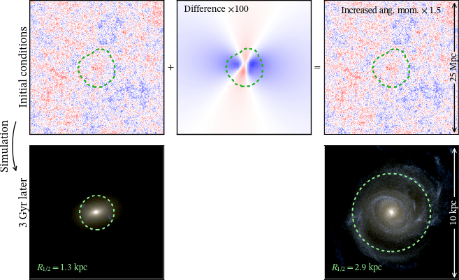
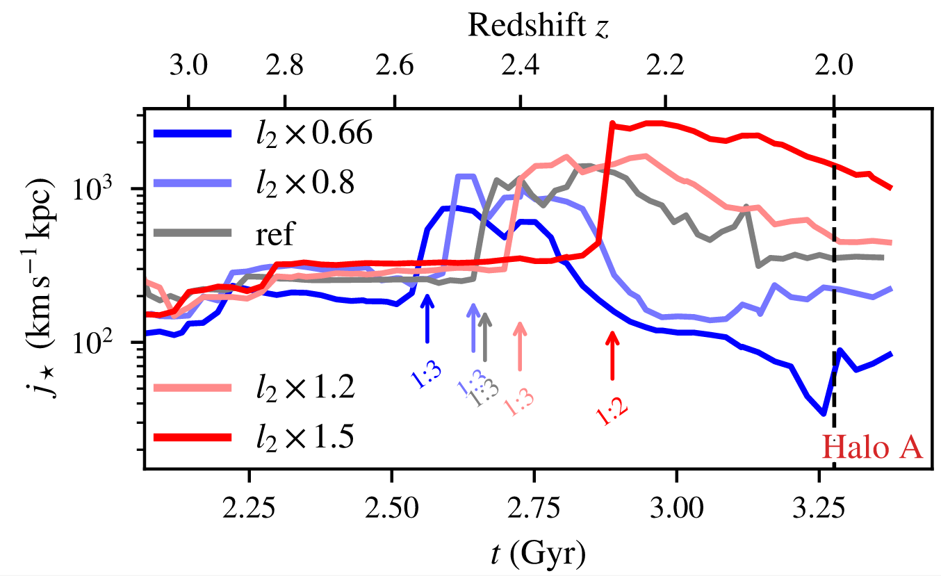
c. Angular momentum GMO

Same galaxy, different tidal enviroment

CC+21b

Study response at low-\(z\)
\(k>10\,h\,\mathrm{Mpc}^{-1}\)

Perturb tides at \(z\rightarrow\infty\)

on \(10-100\,h^{-1}\,\mathrm{Mpc}/h\)

LSS perturbations propagate quasi-linearly down to \(\mathrm{kpc}\) scales

⇒ Large \(k\) contain cosmological information

Part II:
bruteforce solutions

“When everything else fails, use more CPU time”

FLAMINGO (Schaye+23)
\(21\,\mathrm{Gpc}^3\), SWIFT
→ SPH approach

Large-volume hydro-cosmo simulations

State-of-the-art

Millenium-TNG (Springel+22)
\(0.125\,\mathrm{Gpc}^3\), Arepo

→ moving-mesh approach

Grid-based code?

Quite a shame, because it's where France's experts are
(Dubois, Hennebelle, Bournaud, …)

Conclusion & take home message

Possible to build cosmological experiment
⇒ GMs as machine to study scale couplings
- Thoughts on possible applications for DE/DM questions?
- \(10\,\mathrm{Mpc}/h\leftrightarrow \mathrm{kpc}\) for scalars (Mass, \(R_\mathrm{vir}\), ...) is small
- from \(\sim 100\,\mathrm{Mpc}/h\) to \(\sim \mathrm{kpc}\) large for vector quantities (AM, shape)
When clever approaches fail, resort to brute force
- Future is (most likely) driven by GPUs
- Promising developments in France with Dyablo
  https://github.com/Dyablo-HPC/Dyablo

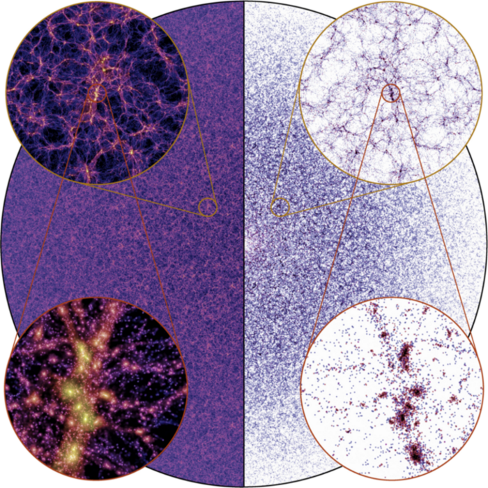
Cosmological simulations

Self-consistent formation of galaxies

Initial conditions

Simulated galaxies

understand:
What's needed to reproduce observations?
explain:
How do galaxies form?
predict:
Future observations?

NASA

\(<1\,\%\)

Exponentially-expanding Universe

Dark matter

Gas (H+He)

Stars

Orders of magnitude

The simulation challenge

Time

Universe: \(13.7\,\mathrm{Gyr}\)
Supernova: \(1\,\mathrm{kyr}\)
⇒ \(10^7\) steps/simulation

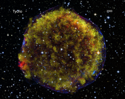
NASA/CXC/A.Jubett

Mass

\(10^{11}\,M_\odot\): Milky-Way
\(1\,M_\odot\): typical star

⇒ \(10^{11}\) particles

Resolution:

\(\sim 10^{6}\,\mathrm{ly}\): cosmological env.
\(\sim 1\,\mathrm{ly}\): supernova scale

⇒ \(>6\) orders of magnitude resolution

⇒ \(10^{18}\) updates

\(230\,\mathrm{yr}\) on my laptop's CPU
\(18\,\mathrm{yr}\) on my GPU
\(11\,\mathrm{month}\) on an NVIDIA H100

Orders of magnitude

of existing code (RAMSES) / Vintergatan simulation

Took:

4 MCPU.hr on 1500 cores (\(490\,\mathrm{yr}\))
\(10^8\) particles + \(3\times10^{8}\) cells (\(M=10^3\,\mathrm{M_\odot}\))
\(67\,\mathrm{GiB}\) of data/output, 200 outputs
Would take the same time on… 6 H100 GPUs

RAMSES: Teyssier 2003
Vintergatan: Cadiou in prep, Agertz+21
Efficiency: green top 500

gas

star

\(\sim 30-70\,\mathrm{Gflop/W}\)

\(\sim 5-50\,\mathrm{Gflop/W}\)

\(\sim2\,\mathrm{tCO_{2,eq}}\)

\(<1\,\mathrm{tCO_{2,eq}}\)?

Dyablo: A New General-Purpose GPU-Accelerated Hydrodynamical Code for Astrophysics

1. Separation of concerns

2. Abstraction

3. Modularity

Dyablo: Overall design

Dyablo: Overall design

Dyablo: Overall design

Dyablo: Implemented physics

Dyablo: how does it scale?

Dyablo: A New General-Purpose GPU-Accelerated Hydrodynamical Code for Astrophysics

3. Modularity

1. Separation of concerns

2. Abstraction

Dyablo: development methods

Dyablo: how does it scale?

dyablo: a (very) promising code

Bottleneck1: communications

Bottleneck1: communications

Bottleneck1: communications

Bottleneck1: communications

Bottleneck2: Reduce communicated data

Bottleneck2: Reduce communicated data

Bottleneck2: Reduce communicated data

Bottleneck2: Reduce communicated data

Bottleneck3: Warp divergences

Bottleneck3: Warp divergences

Bottleneck4: Limited GPU memory

Bottleneck4: Limited GPU memory

Bottleneck4: Limited GPU memory

Bottleneck4: Limited GPU memory

Bottleneck4: Limited GPU memory

Dyablo: status

Part I: (somewhat) clever solutions

Genetic Modification Method (GM)

a. Inverted Initial Conditions

b. Splicing Technique

b. Splicing Technique

b. Splicing Technique

b. Splicing Technique

c. Angular momentum GMO

Part II: bruteforce solutions

Large-volume hydro-cosmo simulations

State-of-the-art

Conclusion & take home message

Cosmological simulations

Orders of magnitude

Orders of magnitude

Dyablo:
A New General-Purpose
GPU-Accelerated
Hydrodynamical Code for Astrophysics

Dyablo:
A New General-Purpose
GPU-Accelerated
Hydrodynamical Code for Astrophysics

Part I:
(somewhat) clever solutions

Part II:
bruteforce solutions