PhD Defense
Kevin Song
2024-12-09
Detecting and Quantifying Entropy Production in Microscopic Systems
What is the nature of this motion?
© Koshu Endo, GeoJapanCorporation 2014
- Does the motion arise from some type of life?
- Is the motion random or deterministic?
- Do the statistical properties of the motion change over time, or do they remain the same?
- Does the motion arise from some type of life?
- Is the motion random or deterministic?
- Do the statistical properties of the motion change over time, or do they remain the same?
Robert Brown, for whom this motion is named, initially thought that this was due to a driving life force.
Repeated experiments with coal dust showed that this was not the case.
Not Alive
Alive
Is there some principled way to tell which process is alive?
How do we define "alive"?
How do we define "alive"?
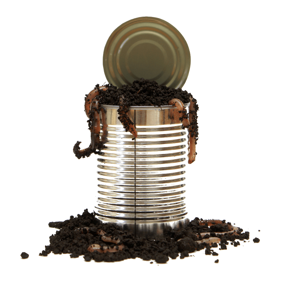
How do we define "alive"?
Fuel
Living Thing
Entropy
Entropy
Entropy
Work
How do we define "alive"?
Fuel (Food)
Living Thing
Entropy
Entropy
Entropy
Work
This definition has several downsides: for example, cars and fires are considered "alive".
But it has enough utility in other situations (not just alive/not-alive decisions) that we'll use it for this talk.

Not Alive
Alive
is alive?
Is there some principled way to tell which process
Not Alive
Alive
is alive?
Is there some principled way to tell which process
produces entropy?
How can we tell if a process produces entropy?
The second law of thermodynamics says that entropy increases over time.
We intuitively use this law all the time to make judgements about the direction of time.
How can we tell if a process produces entropy?
If a process does not produce entropy, there is no time asymmetry
Produces entropy
Does not produce entropy
A process generates entropy if we can distinguish it from its time-reversal
We can also talk about degrees of entropy production

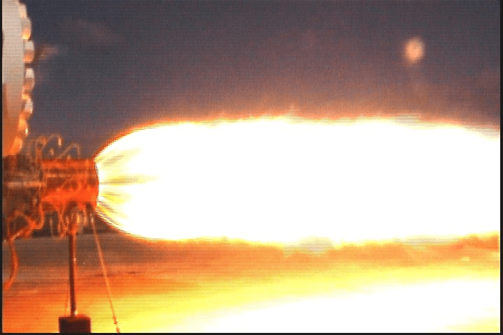
Would like to quantify how irreversible a process is!
Microscopic systems are stochastic in nature.
Can be mathematically described by a stochastic process.
A set of random variables indexed by a time variable \(i \in \mathcal{T}\), with outcome space \(\mathcal{X}\).
We'll focus on discrete-time, discrete-space processes.
We cannot observe stochastic processes directly
denotes that \(x\) is sampled from the stochastic process \(\{X_t\}\) (brackets dropped for simplicity).
Most of the time, we do not know the actual probabilities of the stochastic process (i.e. \(\{X_t\}\) is hidden).
Space of first frame of ink-mixing videos
Space of all ink-mixing videos
Space of second frame of ink mixing videos
A specific first frame of an ink mixing video
A specific second frame of an ink mixing video
A specific ink mixing video (multiple frames)
Process Prefix
A superscript \(\tau\) on a stochastic process denotes the length-\(\tau\) prefix of that process.
Physically, means "stopping the clock" after \(\tau\) time.
Notational Note
We often use formulas that require us to sum over all possible realizations of a stochastic process, e.g.
When possible, I'll instead write this:
Time-Reversal
We denote the time-reversal of a stochastic process \(X_t\) by \(\theta(X_t)\).
Example:
Entropy Production
To find the entropy production, compute the KL Divergence between the forward and reverse processes.
Jarzynski, C. 1997. “Nonequilibrium Equality for Free Energy Differences.” Physical Review Letters 78 (14): 2690.
Crooks, G. E. 1999. “Entropy Production Fluctuation Theorem and the Nonequilibrium Work Relation for Free Energy Differences.” Physical Review. E. 60 (3): 2721–26.
Kawai, R., J. M. R. Parrondo, and C. Van den Broeck. 2007. “Dissipation: The Phase-Space Perspective.” Physical Review Letters 98 (8): 080602.
A significant line of work started by Jarzynski and Crooks in the late 90s leads to the following definition of entropy production:
Sanity check: more KLD = more entropy production
Given samples of \(X_t\) and \(\theta(X_t)\)
Microscopic systems usually obey a property called the Markov property.
We can use this to massively simplify the evaluation of this formula!
Exploiting The Markov Property
Markov Modeling
A stochastic process is Markov (or has the Markov property) iff
This says that each random variable only depends on the previous one.
Markov
Not Markov!
Evaluating KL Divergence with Markov Assumption
Evaluating KL Divergence with Markov Assumption
Evaluating KL Divergence with Markov Assumption
Evaluating KL Divergence with Markov Assumption
If process is Markov, the probability of seeing \(x_1\) after \(x_0\) only depends on \(x_0\).
The probability of seeing \(x_2\) after \(x_1\) only depends on \(x_1\).
Evaluating KL Divergence with Markov Assumption
If process is Markov, the probability of seeing \(x_1\) after \(x_0\) only depends on \(x_0\).
The probability of seeing \(x_2\) after \(x_1\) only depends on \(x_1\).
Evaluating KL Divergence with Markov Assumption
Instead of having to estimate joint probabilities, we only have to estimate pairwise probabilities!
If process is Markov, the probability of seeing \(x_1\) after \(x_0\) only depends on \(x_0\).
The probability of seeing \(x_2\) after \(x_1\) only depends on \(x_1\).
Evaluating KL Divergence with Markov Assumption
Evaluating KL Divergence with Markov Assumption
Suppose \(\mathcal{X} = \{1,2,3\}\) and our system is Markov. Let's pull a very long sample from \(\theta(X_t)\).
Evaluating KL Divergence with Markov Assumption
We will see certain transitions (e.g. \(\color{orange}1\color{black} \rightarrow \color{green}2\)) with a certain probability \(p\).
Evaluating KL Divergence with Markov Assumption
We will see certain transitions (e.g. \(\color{orange}1\color{black} \rightarrow \color{green}2\)) with a certain probability \(p\).
Evaluating KL Divergence with Markov Assumption
We will see certain transitions (e.g. \(\color{orange}1\color{black} \rightarrow \color{green}2\)) with a certain probability \(p\).
If we reverse this sample, we get a sample from \(X_t\).
Evaluating KL Divergence with Markov Assumption
We will see certain transitions (e.g. \(\color{orange}1\color{black} \rightarrow \color{green}2\)) with a certain probability \(p\).
If we reverse this sample, we get a sample from \(X_t\).
Evaluating KL Divergence with Markov Assumption
We will see certain transitions (e.g. \(\color{orange}1\color{black} \rightarrow \color{green}2\)) with a certain probability \(p\).
Note that \( \color{green}2\color{black} \rightarrow \color{orange}1 \) occurs with the same frequency in \(X_t\) as \(\color{orange}1\color{black} \rightarrow \color{green}2\) occurs in \(\theta(X_t)\).
If we reverse this sample, we get a sample from \(X_t\).
Evaluating KL Divergence with Markov Assumption
If we see a transition \(x \rightarrow y\) with probability \(p\) in \(X_t\), we must see \(y \rightarrow x\) with probability \(p\) in \(\theta(X_t)\).
Evaluating KL Divergence with Markov Assumption
1. All probabilities factors into pairwise conditional probabilites
2. We can explicitly compute probabilities in \(p(\theta(X_t^\tau = x))\)
Evaluating KL Divergence with Markov Assumption
where \(p_{ij}\) is the probability to do a transition, and \(\pi_j\) is the probability of being in state \(j\) at a random point in time.
Evaluating KL Divergence with Markov Assumption
- Instead of summing over all length-\(\tau\) trajectories, we're summing over pairs of states.
- \(p_{ij}\) and \(\pi_i\) are easily estimated from data.
- Does not require explicit computations on the reverse process.
What could go wrong?
Molecular systems are small!
In practice, we usually cannot obtain samples from \(X_t\).
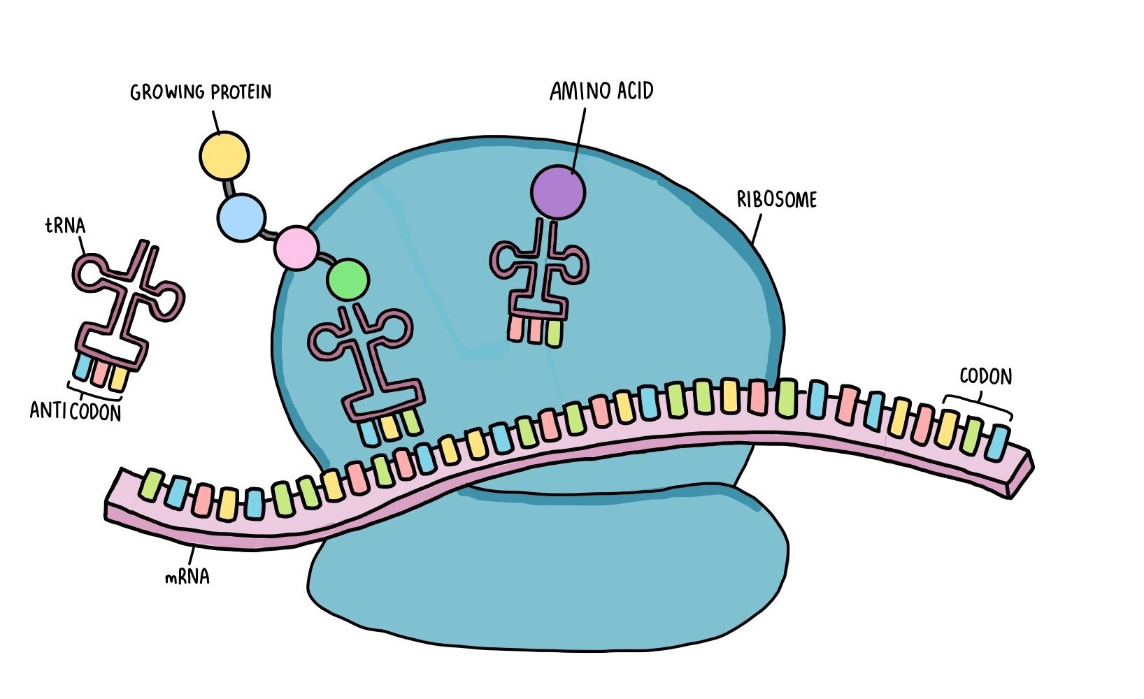

Given this image, we might say a reasonable model for the translation process is a linear chain of states (RNA) and the region currently in the ribosome.
But RNA is really small! We can't accurately resolve which bases are being read.
How can this affect our entropy production estimates?
\(\approx\) 150 bases
Camera View
True System
Coarse-graining gives rise to non-Markov behavior!
Camera View
True System
Coarse-graining gives rise to non-Markov behavior!
Camera View
True System
Coarse-graining gives rise to non-Markov behavior!
Camera View
True System
Coarse-graining gives rise to non-Markov behavior!
Camera View
True System
Coarse-graining gives rise to non-Markov behavior!
Now that we've just seen a state change on the camera, are we more likely to see the particle continue through to the next state, or return to the old state?
Camera View
True System
Coarse-graining gives rise to non-Markov behavior!
Now that we've just seen a state change on the camera, are we more likely to see the particle continue through to the next state, or return to the old state?
Camera View
True System
Now that we've just seen a state change on the camera, are we more likely to see the particle continue through to the next state, or return to the old state?
Continue through
Coarse-graining gives rise to non-Markov behavior!
Camera View
True System
Now that we've just seen a state change on the camera, are we more likely to see the particle continue through to the next state, or return to the old state?
Continue through
Return
Coarse-graining gives rise to non-Markov behavior!
Camera View
True System
Now that we've just seen a state change on the camera, are we more likely to see the particle continue through to the next state, or return to the old state?
Continue through
Return
Appears that particle remembers its old state. But this is non-Markov!
Coarse-graining gives rise to non-Markov behavior!
Even though the underlying physical process \(X_t\) is Markov, our observations \(Y_t\) almost never form a Markov process.
Thesis chapters 2-4 cover how to detect if \(Y_t\) is non-Markov and give one way to quantify its degree of non-Markovianity.
Sneak peek: chapter 5 solves this problem in certain systems by discarding additional information from the coarse-grained observations.
But doesn't tell us what to do instead!
Detecting Entropy Production
Existing Techniques
- TUR
- Ziv-Merhav
- Hidden Markov Modeling
Thermodynamic Uncertainty Relation(s)
Barato, Andre C., and Udo Seifert. 2015. “Thermodynamic Uncertainty Relation for Biomolecular Processes.” Physical Review Letters 114 (April): 158101.
Intuition: molecular systems tend to look very random. The less random they look, the stronger a hidden driving force must be.
This driving force must produce entropy.
Thermodynamic Uncertainty Relation(s)
The original TUR was only proven correct on discrete unicyclic systems, but various extensions have been developed for hierachical coarse-graining, continuous systems, etc.
- Skinner, Dominic J., and Jörn Dunkel. 2021. “Improved Bounds on Entropy Production in Living Systems.” Proceedings of the National Academy of Sciences of the United States of America 118 (18)
- Knotz, Gabriel, Till Moritz Muenker, Timo Betz, and Matthias Krüger. 2024. “Entropy Bound for Time Reversal Markers.” Frontiers in Physics 11 (February): 1331835.
- Bisker, Gili, Matteo Polettini, Todd R. Gingrich, and Jordan M. Horowitz. 2017. “Hierarchical Bounds on Entropy Production Inferred from Partial Information.” Journal of Statistical Mechanics 2017 (9): 093210.
- Dechant, Andreas, and Shin-Ichi Sasa. 2021. “Continuous Time Reversal and Equality in the Thermodynamic Uncertainty Relation.” Phys. Rev. Research 3 (4): 042012.
- Di Terlizzi, I., M. Gironella, D. Herraez-Aguilar, T. Betz, F. Monroy, M. Baiesi, and F. Ritort. 2024. “Variance Sum Rule for Entropy Production.” Science (New York, N.Y.) 383 (6686): 971–76.
Primary downside: only provides a lower bound on entropy production!
Secondary downside: behavior of bounds not well understood under coarse-graining (Knotz 2024).
Ziv-Merhav Compression
The Kullback-Leibler Divergence is more common in information theory and machine learning.
There is a way to compute \(D_{KL}\) which is based on information-theoretic techniques.
Ziv-Merhav Compression
Suppose I draw some observations \(x_1 \dots x_n \sim X\). I want to transmit these observations to someone else.
I need to use some minimum number of bits to transmit these \(n\) observations. What is this minimum?


Requires \(N H(X)\) bits!
Ziv-Merhav Compression
Suppose I draw some observations \(x_1 \dots x_n \sim X\). I want to transmit these observations to someone else.
I need to use some minimum number of bits to transmit these \(n\) observations. What is this minimum?


Requires \(N H(X)\) bits!
Ziv-Merhav Compression
Now suppose I draw \(\color{red}y_1 \dots y_n \sim Y\). How many bits do I need to transmit these observations if I use a code which is optimal for \(X\)?
Number of bits needed to encode \(Y\) using a code for \(X\).
Number of bits needed to encode \(Y\) using a code for \(Y\).
Ziv-Merhav Cross-Parsing
Goal: Encode \(Y\) using phrases from \(X\).
Ziv, J., and N. Merhav. 1993. “A Measure of Relative Entropy between Individual Sequences with Application to Universal Classification.” IEEE Transactions on Information Theory / Professional Technical Group on Information Theory 39 (4): 1270–79.
Ziv-Merhav Cross-Parsing
Ziv-Merhav Cross-Parsing
Ziv-Merhav Cross-Parsing
Ziv-Merhav Cross-Parsing
Ziv-Merhav Cross-Parsing
Ziv-Merhav Cross-Parsing
Ziv-Merhav Cross-Parsing
Using this encoding of \(y\), we can estimate \(H(Y, X)\).
1. Draw sample from \(X_t\).
1. Draw sample from \(X_t\).
2. Reverse to obtain sample from \(\theta(X_t)\).
1. Draw sample from \(X_t\)
2. Reverse to obtain sample from \(\theta(X_t)\)
3. Compute Ziv-Merhav cross parse and estimate \(H(X, \theta(X))\)
1. Draw sample from \(X_t\)
2. Reverse to obtain sample from \(\theta(X_t)\)
3. Compute Ziv-Merhav cross parse and estimate \(H(X, \theta(X))\)
4. Estimate \(H(X_t)\) using methods discussed in Chapter 2 of thesis.
1. Draw sample from \(X_t\)
2. Reverse to obtain sample from \(\theta(X_t)\)
3. Compute Ziv-Merhav cross parse and estimate \(H(X, \theta(X))\)
4. Estimate \(H(X_t)\) using methods discussed in Chapter 2 of thesis.
4. Combine these two quantities to estimate \(D_{KL}\).
1. Draw sample from \(X_t\)
2. Reverse to obtain sample from \(\theta(X_t)\)
3. Compute Ziv-Merhav cross parse and estimate \(H(X, \theta(X))\)
4. Estimate \(H(X_t)\) using methods discussed in Chapter 2 of thesis.
4. Combine these two quantities to estimate \(D_{KL}\).
5.Plug this estimate into the formula for entropy production.
Downsides: Requires lots of data, inference time, convergence unknown
Upsides: No modeling choices, just shove data into the estimator and crank
Hidden Markov Models
A Markov model where we don't get to explicitly see the state.
1
2
3
4
Bouguila, Nizar, Wentao Fan, and Manar Amayri, eds. 2022. Hidden Markov Models and Applications. 1st ed. Unsupervised and Semi-Supervised Learning. Cham, Switzerland: Springer Nature.
Actual State
1
Observation
A
Hidden Markov Models
A Markov model where we don't get to explicitly see the state.
1
2
3
4
Bouguila, Nizar, Wentao Fan, and Manar Amayri, eds. 2022. Hidden Markov Models and Applications. 1st ed. Unsupervised and Semi-Supervised Learning. Cham, Switzerland: Springer Nature.
Actual State
12
Observation
AA
Hidden Markov Models
A Markov model where we don't get to explicitly see the state.
1
2
3
4
Bouguila, Nizar, Wentao Fan, and Manar Amayri, eds. 2022. Hidden Markov Models and Applications. 1st ed. Unsupervised and Semi-Supervised Learning. Cham, Switzerland: Springer Nature.
Actual State
121
Observation
AAB
Hidden Markov Models
A Markov model where we don't get to explicitly see the state.
1
2
3
4
Bouguila, Nizar, Wentao Fan, and Manar Amayri, eds. 2022. Hidden Markov Models and Applications. 1st ed. Unsupervised and Semi-Supervised Learning. Cham, Switzerland: Springer Nature.
Actual State
1212
Observation
AABA
| State | P("A") | P("B") |
|---|---|---|
| 1 | ||
| 2 | ||
| 3 | ||
| 4 |
1
2
3
4
Observed
AABBAB
| State | P("A") | P("B") |
|---|---|---|
| 1 | ||
| 2 | ||
| 3 | ||
| 4 |
Inputs
Outputs
- Dynamics of hidden states (usually as a graph)
- Observed sequence of states
- Markov transition probabilities
- Probabilities of observing outcomes in each hidden state
What happens if we specify the wrong graph?
Graph given to algorithm
Actual Graph
1
2
3
4
3
2
1
4
5
Prior Work Summary
| Method | Advantage | Disadvantage |
|---|---|---|
| TUR | Straightforward to apply Fast |
Only provides lower bound |
| Ziv-Merhav | No parameters to set or guess | Computationally expensive, convergence not guaranteed |
| HMM | Easy to understand result Very well-established algorithms |
If wrong graph provided to algorithm, results may be garbage |
| Markov Formula | Fast, easy,correct | Cannot be used when data is non-Markov |
Blom, Kristian, Kevin Song, Etienne Vouga, Aljaž Godec, and Dmitrii E. Makarov. 2024. “Milestoning Estimators of Dissipation in Systems Observed at a Coarse Resolution.” Proceedings of the National Academy of Sciences of the United States of America 121 (17): e2318333121.
Milestoning Estimators of Dissipation in Systems Observed at a Coarse Resolution
Joint work with Kristian Blom, Aljaž Godec, Dmitrii Makarov, and Etienne Vouga, published in PNAS.
Getting Better Results By Throwing Out That Pesky Data
Single File Diffusion

Single File Diffusion

Single File Diffusion

Single File Diffusion

Single File Diffusion

Single File Diffusion

We can only see a single tracer particle (indicated in red).

Number of vacancies and overall sites can vary.
Stronger bias = more entropy production
Only being able to see a single tracer particle induces coarse-graining on the system.
Only being able to see a single tracer particle induces coarse-graining on the system.


?
?
?
?
?
?

A
B
C
D
1
2
3
Milestoning
In my proposal, I discussed a technique called milestoning. It allowed us to make highly non-Markov systems look Markov while preserving important elements of the behavior.
We're going to use this technique again for entropy production estimation, but it's going to look slightly different in a discrete system.
= pixel
= milestone pixel
We are given a system which is already lumped. We can only tell which lump(pixel) a particle is in, not the microscopic state.
1
2
3
4
5
6
7
8
9
We (the data analysis team) designate several lumps(pixels) as milestones.
1
2
3
4
5
6
7
8
9
= pixel
= milestone pixel
In the milestoned trajectory, we only record a milestone state if this is the first time at this milestone since visiting a different milestone.
1
2
3
4
5
6
7
8
9
= pixel
= milestone pixel
In the milestoned trajectory, we only record milestone states, and only if this is the first time at this milestone since visiting a different milestone.
1
2
3
4
5
6
7
8
9
Lumped Trajectory
Milestoned Trajectory
4
4
= pixel
= milestone pixel
1
2
3
4
5
6
7
8
9
Lumped Trajectory
Milestoned Trajectory
4 5
4
= pixel
= milestone pixel
1
2
3
4
5
6
7
8
9
Lumped Trajectory
Milestoned Trajectory
4 5
4
= pixel
= milestone pixel
1
2
3
4
5
6
7
8
9
Lumped Trajectory
Milestoned Trajectory
4 5
4
= pixel
= milestone pixel
1
2
3
4
5
6
7
8
9
Lumped Trajectory
Milestoned Trajectory
4 5 6
4 6
= pixel
= milestone pixel
1
2
3
4
5
6
7
8
9
Lumped Trajectory
Milestoned Trajectory
4 5 6 5
4 6
= pixel
= milestone pixel
1
2
3
4
5
6
7
8
9
Lumped Trajectory
Milestoned Trajectory
4 5 6 5 6
4 6
= pixel
= milestone pixel
1
2
3
4
5
6
7
8
9
Lumped Trajectory
Milestoned Trajectory
4 5 6 5 6
4 6
= pixel
= milestone pixel
1
2
3
4
5
6
7
8
9
Lumped Trajectory
Milestoned Trajectory
4 5 6 5 6
4 6
= pixel
= milestone pixel
1
2
3
4
5
6
7
8
9
Lumped Trajectory
Milestoned Trajectory
4 5 6 5 6 7
4 6
= pixel
= milestone pixel
1
2
3
4
5
6
7
8
9
Lumped Trajectory
Milestoned Trajectory
4 5 6 5 6 7 6
4 6
= pixel
= milestone pixel
1
2
3
4
5
6
7
8
9
Lumped Trajectory
Milestoned Trajectory
4 5 6 5 6 7 6
4 6
= pixel
= milestone pixel
1
2
3
4
5
6
7
8
9
Lumped Trajectory
Milestoned Trajectory
4 5 6 5 6 7 6
4 6
= pixel
= milestone pixel
1
2
3
4
5
6
7
8
9
Lumped Trajectory
Milestoned Trajectory
4 5 6 5 6 7 6 5
4 6
= pixel
= milestone pixel
1
2
3
4
5
6
7
8
9
Lumped Trajectory
Milestoned Trajectory
4 5 6 5 6 7 6 5 6
4 6
= pixel
= milestone pixel
1
2
3
4
5
6
7
8
9
Lumped Trajectory
Milestoned Trajectory
4 5 6 5 6 7 6 5 6 5
4 6
= pixel
= milestone pixel
1
2
3
4
5
6
7
8
9
Lumped Trajectory
Milestoned Trajectory
4 5 6 5 6 7 6 5 6 5
4 6
= pixel
= milestone pixel
1
2
3
4
5
6
7
8
9
Lumped Trajectory
Milestoned Trajectory
4 5 6 5 6 7 6 5 6 5
4 6
= pixel
= milestone pixel
1
2
3
4
5
6
7
8
9
Lumped Trajectory
Milestoned Trajectory
4 5 6 5 6 7 6 5 6 5 4
4 6 4
= pixel
= milestone pixel


Lumps (i.e. pixels or other coarse-graining units) are usually fixed by experimental limitations. Milestones are chosen during data processing.
These are all valid milestoning schemes!
Where transition probabilities \(p\) are estimated directly from the data, either using a lumped trace or a lumped + milestoned trace.


Lumped Trajectory
Milestoned Trajectory
4 5 6 5 6 7 6 5 6 5 4
4 6 4
[
| 1 | |

Lumped Trajectory
Milestoned Trajectory
4 5 6 5 6 7 6 5 6 5 4
4 6 4
[
| 2 | |

Lumped Trajectory
Milestoned Trajectory
4 5 6 5 6 7 6 5 6 5 4
4 6 4
[
| 2 | |
| 1 | |

Lumped Trajectory
Milestoned Trajectory
4 5 6 5 6 7 6 5 6 5 4
4 6 4
[
| 3 | |
| 1 | |

Lumped Trajectory
Milestoned Trajectory
4 5 6 5 6 7 6 5 6 5 4
4 6 4
| 5 | |
| 4 | |
[

Lumped Trajectory
Milestoned Trajectory
4 5 6 5 6 7 6 5 6 5 4
4 6 4
| 5 | |
| 4 | |
| 1 | |
[

Lumped Trajectory
Milestoned Trajectory
4 5 6 5 6 7 6 5 6 5 4
4 6 4
| 5 | |
| 4 | |
| 1 | |
[

Lumped Trajectory
Milestoned Trajectory
4 5 6 5 6 7 6 5 6 5 4
4 6 4
| 5 | |
| 4 | |
| 2 | |
| 2 |
[
| 5 | |
| 4 | |
| 2 | |
| 2 |

Lumped Trajectory
4 5 6 5 6 7 6 5 6 5 4
| 5 | |
| 4 | |
| 2 | |
| 2 |
| 5 | |
| 4 | |
| 2 | |
| 2 |
Lumped Trajectory
4 5 6 5 6 7 6 5 6 5 4
| 5 | |
| 4 | |
| 2 | |
| 2 |
| 0.55 | |
| 0.44 | |
| 0.22 | |
| 0.22 |


Lumped Trajectory
4 5 6 5 6 7 6 5 6 5 4
| 5 | |
| 4 | |
| 2 | |
| 2 |
| 0.55 | |
| 0.44 | |
| 0.22 | |
| 0.22 |

\(Q\): Ratio of estimated entropy production to true entropy production.
Ideally, \(Q = 1.0\).


Conclusion: across different types of dynamics and estimators, it is better to milestone than not-milestone, even though we throw out some information.


Chapter 5 Additional Results
Chapter 5 of the thesis discusses additional results that demonstrate how removing information can result in better entropy production estimates, including:
- Spacing milestones far apart gives better estimates than milestones close together
- The time the tracer spends between milestones must be ignored to get the correct entropy production for single-file diffusion. (This is not true in general).
- Additional details on the correctness time-reversal and practicalities of milestoning.
Practical Evaluations of Entropy Production
Information-theoretical limit on the estimates of dissipation by molecular machines using single-molecule fluorescence resonance energy transfer experiments
Joint work with Dmitrii Makarov, and Etienne Vouga, published in JCP
Song, Kevin, Dmitrii E. Makarov, and Etienne Vouga. 2024. “Information-Theoretical Limit on the Estimates of Dissipation by Molecular Machines Using Single-Molecule Fluorescence Resonance Energy Transfer Experiments.” The Journal of Chemical Physics 161 (4): 044111.
Chapter 6 of thesis

We can't take (optical) videos of these processes.
Instead, if we want to track (some limited) information about positions over time, we can use Förster resonance energy transfer (FRET).
FRET Model

Some complex physics (including a term that scales as \(x^6\), but a very straightforward interpretation.
FRET Model

FRET Model

Our goal will be to predict the entropy production of the walker.
FRET Model

We have a flashbulb which goes off at random times.
We can control how often this light flashes per second (on average) with a system parameter \(\mu\).
Every time the flashbulb goes off, we see the color of the state, but not what state it came from.

FRET Model
Time
What We See
The system could have transitioned from orange to purple to green here, but we can't see it because our flashbulb didn't go off!
Given this photon sequence, how can we estimate the entropy production of the walker?
We can assume Markov behavior and write down a formula for the entropy production
In the limit as \(\mu \rightarrow 0\), the entropy production goes to zero.
In the limit as \(\mu \rightarrow \infty\), the entropy production goes to the true value.

Single File Diffusion with Photons
The same single-file diffusion process from earlier, but now we can only observe photon colors!

When the light flashes, we see the color of the site this walker is on.
We cannot observe this walker at all.
How can we estimate the entropy production for this system?
- Plug probabilities in to entropy production formula (like Chapter 5)
- Use Ziv-Merhav estimator
- Use a hidden Markov model
Actual Model
Presumed Model
What happens if we use the wrong model for the HMM?
We call the HMM estimates using the wrong model the "MLE" estimate.


Only tracer particle biased

Both particles biased

Conclusions
- No method gives us ideal entropy production for this (relatively simple) system
- If you know the correct underlying model, hidden Markov modeling is your best technique (not published).
- If you might be wrong about the model, compression (Ziv-Merhav) gives you slightly better results all-around, but still doesn't give the correct entropy production
- Plug-in estimators are probably not the right solution.
But wait, there's more!
...in the thesis.
See Chapter 6 for:
- Equations and derivations of the exact entropy rate for certain systems when measured with photons
- Theory and results for cases when the photon color does not tell us exactly which state we are in
- When there can be error in the photon color
- When three states only emit two colors in total
- Expressions for the exact probabilities of a photon sequence
- What to do about waiting times

Summary
Molecular physics and information theory are related
Throughout my PhD, I have exploited these connections to make various inference algorithms for molecular systems.
| Chapter 2 | Using compression as an entropy rate estimator to infer coarse-graining |
| Chapter 4 | Extending Chapter 2 to continuous-space systems by careful discretization of the state space |
| Chapter 5 | Using the representations of Chapter 4 to improve estimates of entropy production rate |
| Chapter 6 | Estimating entropy rates by various means (including compression) when the state cannot be seen |
Fine Grained
Coarse Grained
Zero Entropy Production
Positive Entropy Production

Open Problem: Entropy-Generating Coarse-Grainings
Fine Grained
Coarse Grained
Zero Entropy Production
Positive Entropy Production

Fine Grained
Coarse Grained
Zero Entropy Production
Positive Entropy Production
Fine Grained
Coarse Grained
Zero Entropy Production
Positive Entropy Production

Fine Grained
Coarse Grained
Zero Entropy Production
Positive Entropy Production
?
If we can show that these do not exist, then any entropy production exhibited by a coarse-grained system must be real!
Fine Grained
Coarse Grained
Zero Entropy Production
Positive Entropy Production
?
Open Problem: Representations
We want to write down this system in a manner that is invariant to rigid transforms.
Open Problem: Representations
Open Problem: Representations
If you actually try this, you get the wrong scaling result for chain entropy vs end-to-end length!
Avinery, Ram, Micha Kornreich, and Roy Beck. 2019. “Universal and Accessible Entropy Estimation Using a Compression Algorithm.” Physical Review Letters 123 (17): 178102.
Avinery et. al.'s representation
Avinery et. al.'s angle definition
Avinery et. al.'s angle definition
These two representations give different answers....but the physics of a system should not depend on the representation used to write it down!
What is going on here?
FIN
We can also have situations where a state outputs mixed colors.


Time
This looks like it started in the orange state, transitioned through the mixed state, and ended in the purple state....but did it?
We'll make a quick comment on the case where each state has a unique color and then move to the more interesting cases.
Reversing a Markov Model
Time
Reversing a Markov Model
Time
Reversing a Markov Model
Time
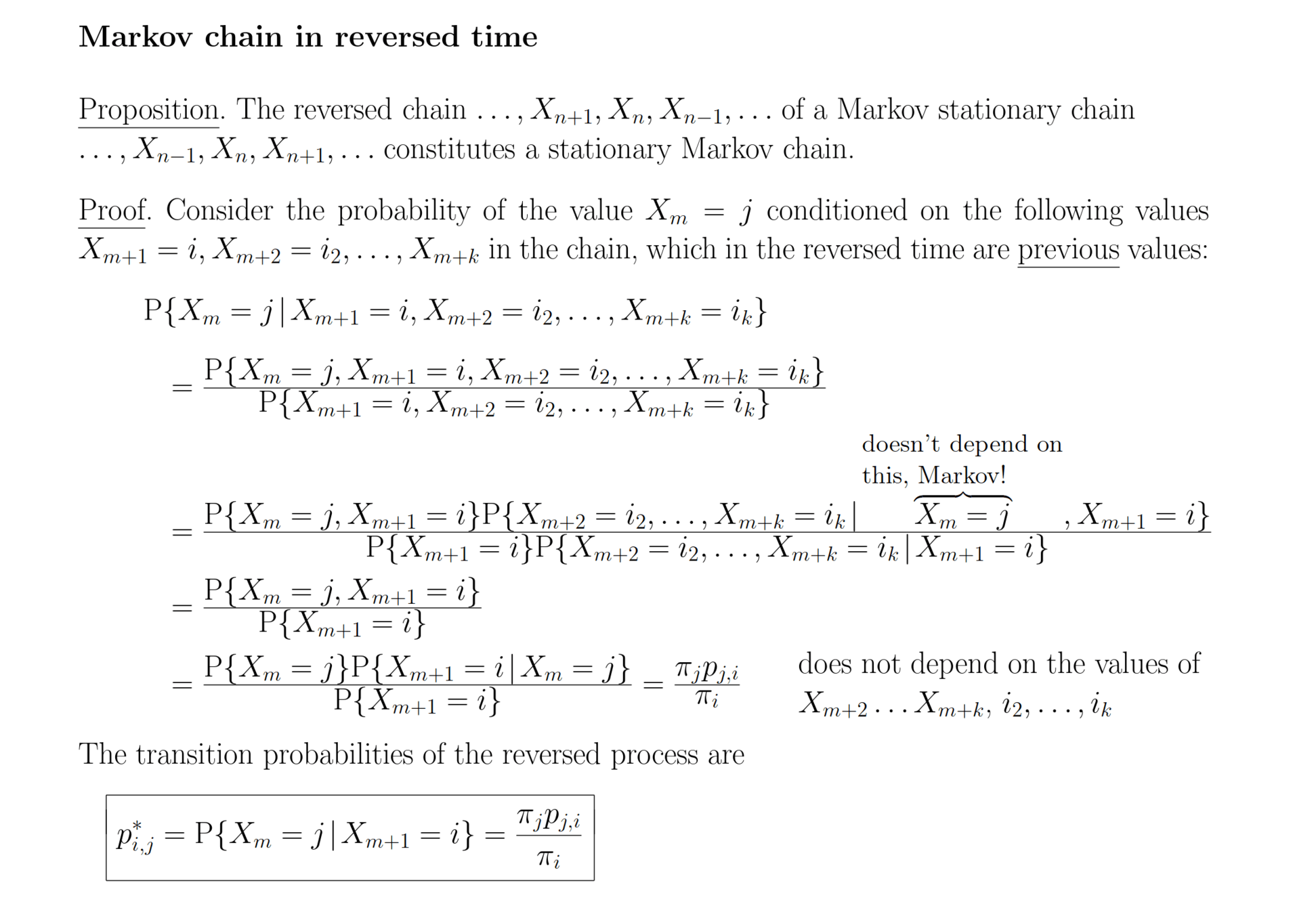
By more carefully analyzing the Markov condition, we find that we cam also reverse the variable dependencies.
Reversing a Markov Model
Time
By more carefully analyzing the Markov condition, we find that we cam also reverse the variable dependencies.
Proof
Reversing a non-Markov Model
Time
Reversing a non-Markov Model
Time
However, without the Markov condition, there is no way to reverse these dependencies anymore. Random variables now depend on future outcomes.
Problems with \(\theta\)
Evaluating \(\theta\)
This is not the correct form of \(\theta\) in general!
Evaluating \(\theta\)
Consider a particle moving around. At each instant in time, we capture its position and momentum.
Evaluating \(\theta\)
Consider a particle moving around. At each instant in time, we capture its position and momentum.
Evaluating \(\theta\)
Consider a particle moving around. At each instant in time, we capture its position and momentum.
Evaluating \(\theta\)
Consider a particle moving around. At each instant in time, we capture its position and momentum.
Evaluating \(\theta\)
Consider a particle moving around. At each instant in time, we capture its position and momentum.
Evaluating \(\theta\)
Consider a particle moving around. At each instant in time, we capture its position and momentum.
Evaluating \(\theta\)
Consider a particle moving around. At each instant in time, we capture its position and momentum.
Evaluating \(\theta\)
Consider a particle moving around. At each instant in time, we capture its position and momentum.
Evaluating \(\theta\)
Consider a particle moving around. At each instant in time, we capture its position and momentum.
This is aphysical nonsense! The ball moves in the opposite direction of its momentum.
The Correct Time Reversal Operator
This is still not general enough!
Complication: Incomplete Observations
Simple Model: Ring

Simple Model: Ring

Simple Model: Ring

Simple Model: Ring

Simple Model: Ring


Coarse-graining can remove all evidence of irreversibility!
However, even if we assume that cycles like these are not completely hidden by coarse-graining, it still introduces other challenges.
PNAS Ring-in-Ring


Lumping of cycles introduces non-Markov behavior, as we have already seen.
will become
We're going to further coarse-grain the trace by milestoning it.
Easy (low entropy)
Hard (high entropy)
Entropy
"How hard is it to guess what happens?"
Entropy Sets a Communication Limit

,
,
Entropy Sets a Communication Limit


Entropy Sets a Communication Limit


Entropy Sets a Communication Limit


Entropy Sets a Communication Limit


Entropy Sets a Communication Limit


Let's say we repeat this process \(N\) times. How many bits do we need to send over the wire?
Entropy Sets a Communication Limit


Let's say we repeat this process \(N\) times. How many bits do we need to send over the wire?
Shannon's source coding theorem
\( H(X) \) bits per observation
Ease of prediction translates to ease of communication!
Entropy sets a communication compression limit
If transmitting \(N\) observations from a process with entropy \(H(X)\), we cannot use fewer than \(N H(X)\) bits.
No compression scheme can use fewer than \(N H(X)\) bits, else we could violate the source coding theorem.
Several compression algorithms achieve this bound!
Altering the Deal


Generally, optimal codes use shorter representations for more frequent symbols and longer representations for less frequent symbols.
So what happens if the frequencies change?


,
,
Altering the Deal


Altering the Deal


Altering the Deal


Altering the Deal


Altering the Deal


How many bits do we need to use to send these observations, drawn from \(Y\), but encoded using an optimal code for \(X\)?
Altering the Deal
Altering the Deal
minimum number of bits
penalty for using a code optimized for \(X\) when we were actually transmitting \(Y\)
Altering the Deal
Altering the Deal
Can be estimated just by compressing \(Y\) using any compression algorithm.
Altering the Deal
Estimated by using a special cross-parse algorithm.
Additional wrinkle: it is better to have milestones far apart than close together
= standard lump
= milestone lump
Additional wrinkle: it is better to have milestones far apart than close together
= standard lump
= milestone lump
The particle just entered a milestone. What is the probability of it returning to its previous milestone versus continuing to the next one?
Additional wrinkle: it is better to have milestones far apart than close together
= standard lump
= milestone lump
6 sites
Additional wrinkle: it is better to have milestones far apart than close together
= standard lump
= milestone lump
6 sites
4 sites
Additional wrinkle: it is better to have milestones far apart than close together
= standard lump
= milestone lump
The particle just entered a milestone. What is the probability of it returning to its previous milestone versus continuing to the next one?
Additional wrinkle: it is better to have milestones far apart than close together
= standard lump
= milestone lump
The particle just entered a milestone. What is the probability of it returning to its previous milestone versus continuing to the next one?
12 sites
Additional wrinkle: it is better to have milestones far apart than close together
= standard lump
= milestone lump
The particle just entered a milestone. What is the probability of it returning to its previous milestone versus continuing to the next one?
12 sites
10 sites
Additional wrinkle: it is better to have milestones far apart than close together
= standard lump
= milestone lump
12 sites
10 sites
Additional wrinkle: it is better to have milestones far apart than close together
= standard lump
= milestone lump
When the milestones are further apart, the milestoned trajectory behaves more and more like the original Markov process.
In the limit of infinite distance, we recover the original process. See Section 5.4 for details.
Additional Wrinkle: Waiting Times
Milestones and lumps both create an additional piece we haven't talked about: waiting times.
TIME
Milestone
Lump
A
B
C
D
1
2
3
A
B
1
A
B
C
2
B
A
1
B
C
2
D
3
Unequal times between milestone crossings!
Waiting times can also contribute to entropy production, e.g. if waiting times systematically increase, this creates an asymmetry in the forward/backward processes.
Additional Wrinkle: Waiting Times
In the system presented here, we show (cf. Section 5.5) that in this case, we must ignore the waiting times in order to obtain the correct entropy production.
However, in other systems studied in the literature (Martínez et. al.), the waiting times do contribute to entropy production.
Martínez, Ignacio A., Gili Bisker, Jordan M. Horowitz, and Juan M. R. Parrondo. 2019. “Inferring Broken Detailed Balance in the Absence of Observable Currents.” Nature Communications 10 (1): 3542.