Christopher Makler
Stanford University Department of Economics
Econ 50: Lecture 14
Resource Constraints and Production Possibilities
Today's Agenda
Part 1: Resource Constraints and the PPF
Part 2: Optimization
The "Desert Island" Model
Resource constraints and the PPF
Deriving the equation of the short-run PPF
Shifts in the PPF
The Marginal Rate of Transformation
Relationship between MPL and MRT
The "Gravitational Pull" argument
Tangency when calculus works
Corners and kinks

The “Desert Island" Model
Economics is the study of how
we use scarce resources
to satisfy our unlimited wants
Resources
Goods
Happiness
🌎
⌚️
🤓

Production functions
Utility functions
Demand
Supply
Equilibrium
🤩
🏪
⚖
Wednesday: Little Green Pieces of Paper
Multiple Uses of Resources
Labor
Fish
🐟
Coconuts
🥥
[GOOD 1]
⏳
[GOOD 2]
Resource Constraint
Production Possibilities
Resource Constraint
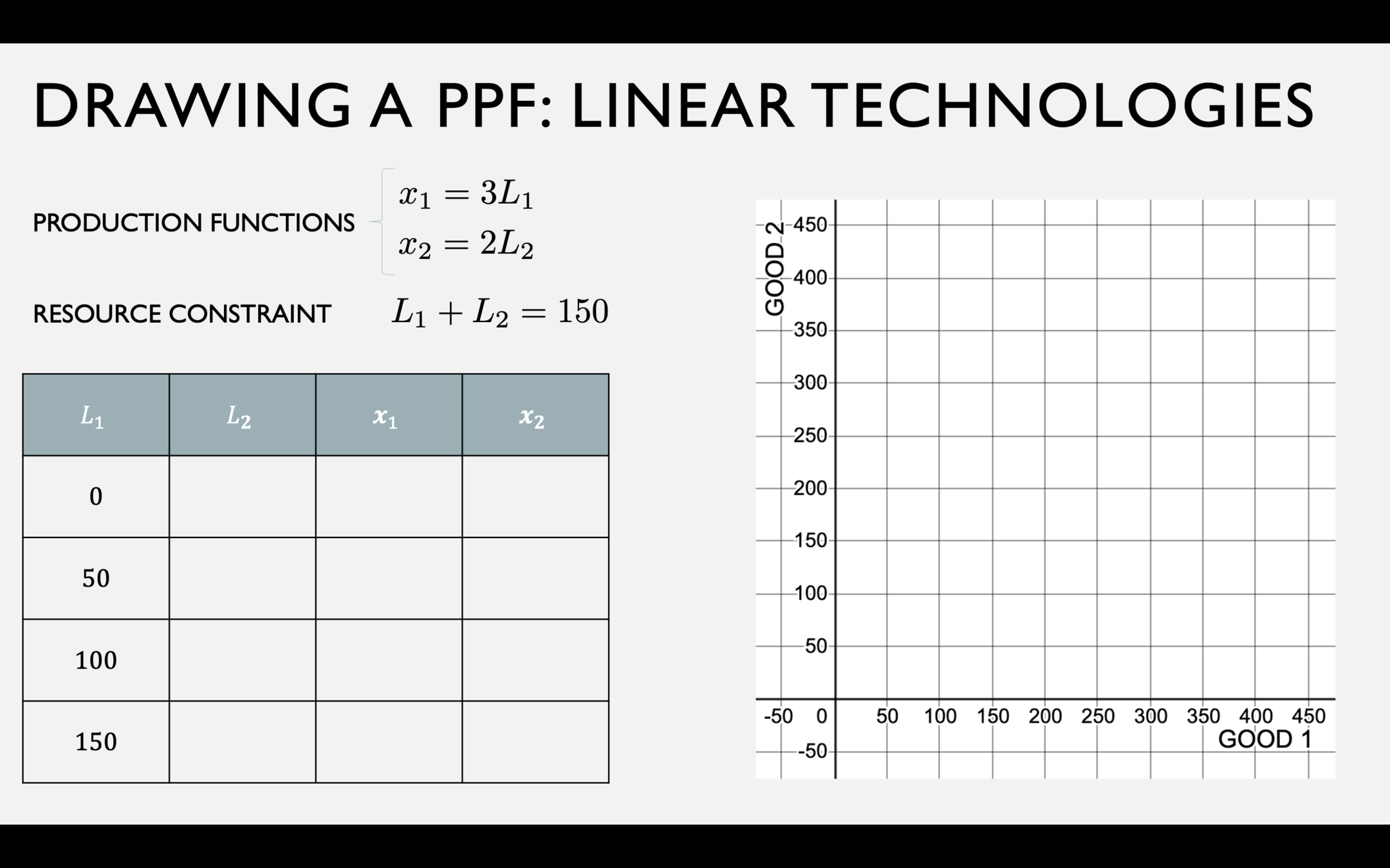

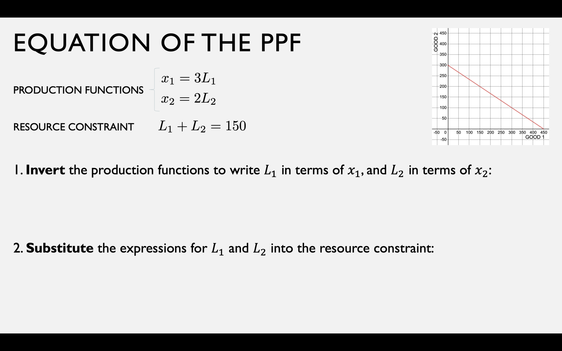
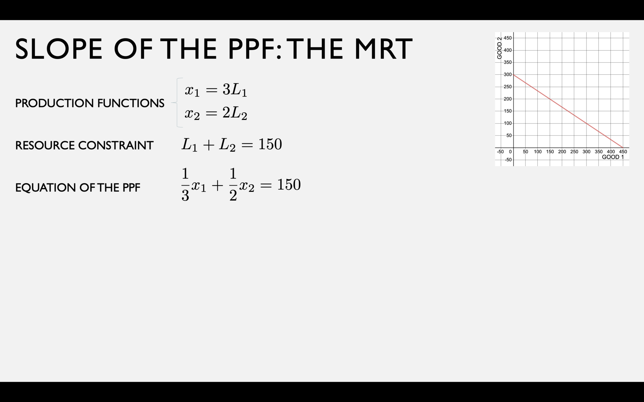
A PPF with Linear Technologies
Fish production function
Coconut production function
Resource Constraint
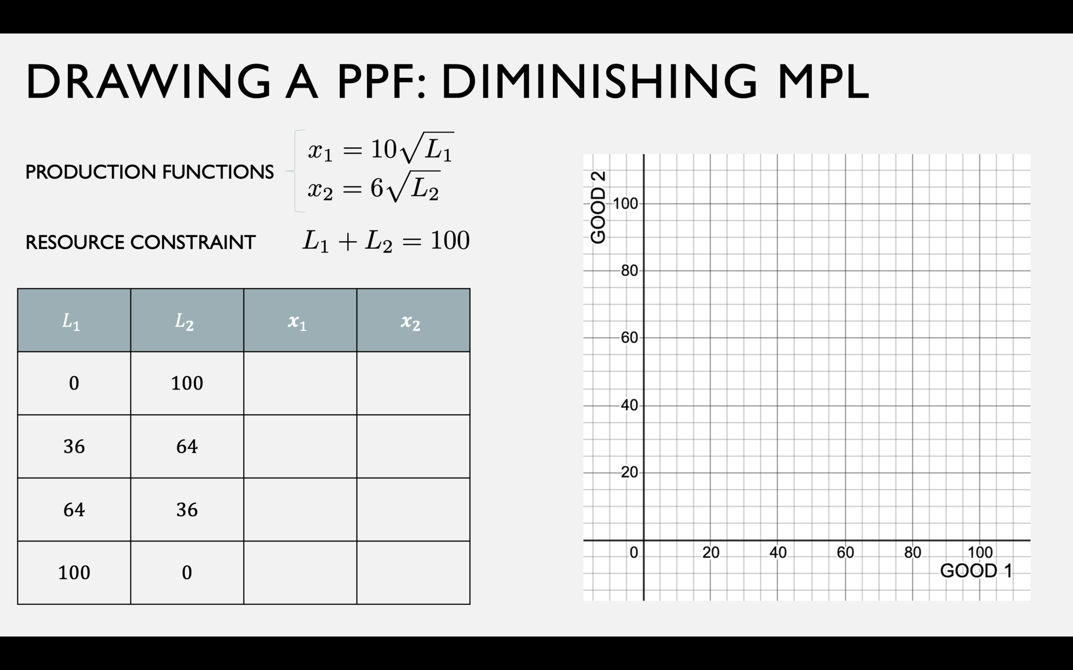

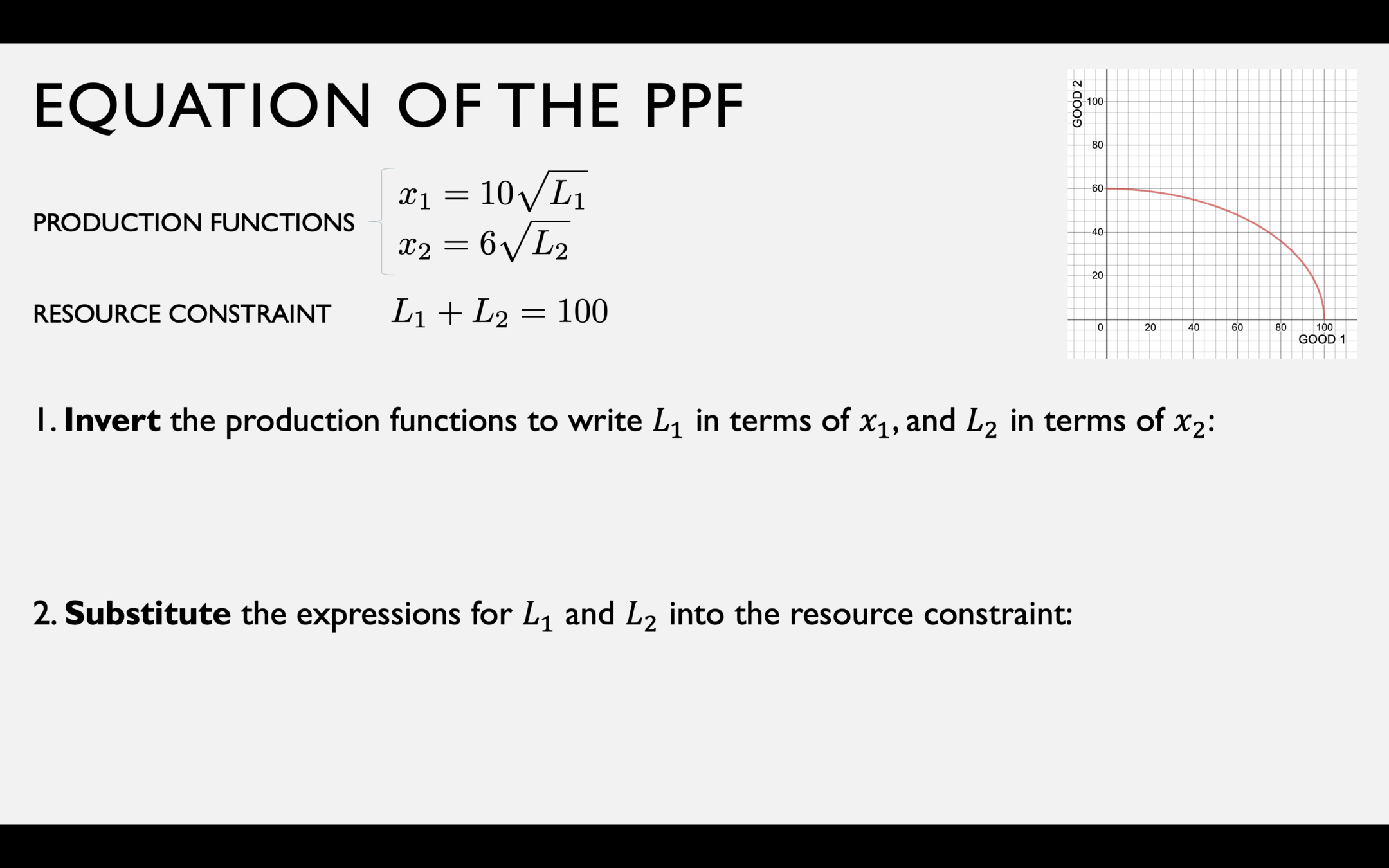
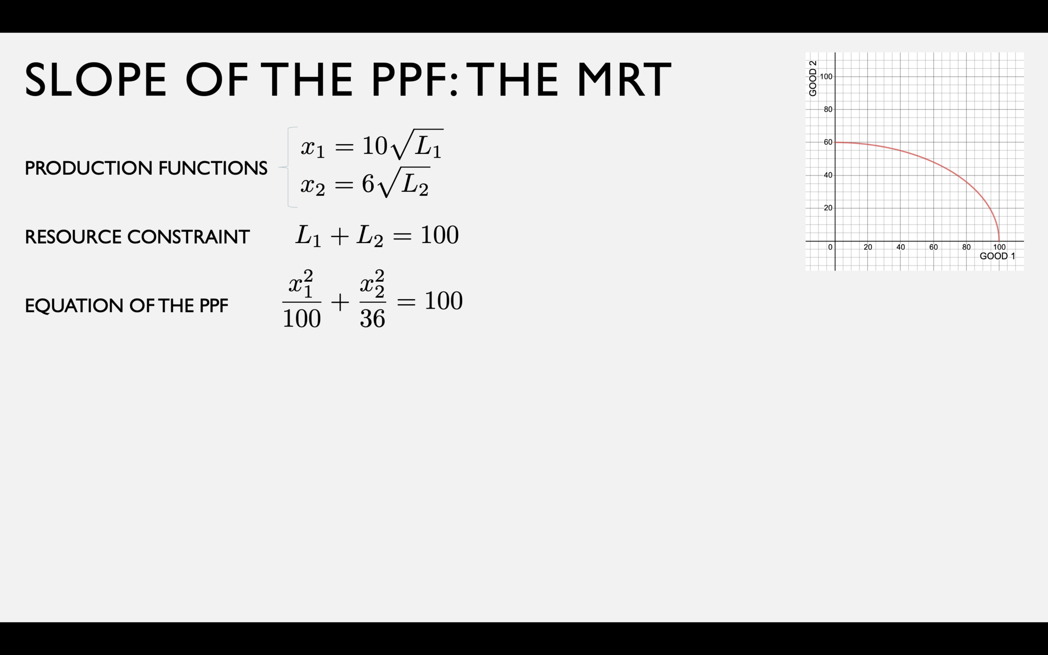
A PPF with Diminishing \(MP_L\)
Fish production function
Coconut production function
Resource Constraint
- Suppose we want to produce a lot more of something -- ventilators, masks, toilet paper, hand sanitizer
- Some resources can be reallocated quickly; others are more specialized and can't be quickly repurposed
- How can we "scale up" in the short run and the long run?
- How do short-run tradeoffs compare with long-run tradeoffs?
Shifts in the PPF
Consider an economy with \(\overline L = 100\) units of labor and \(\overline K = 100\) units of capital.
In the short run, \(K_1 = 64\) and \(K_2 = 36\).
In the long run, capital can be reallocated in any combination between goods 1 and 2.
Max in SR
Max in LR
- Up to now: how a short-run PPF can shift due to changing the allocation of capital, holding production functions constant.
- What happens when the technology itself (i.e. the production function) changes?
Improvements in Technology
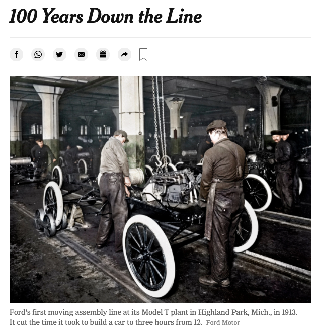
The New York Times, Oct. 29, 2013
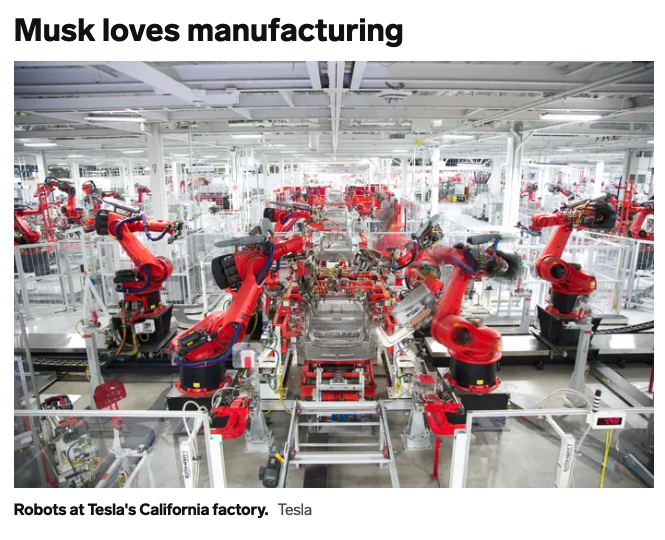
Insider, July 23, 2020
Consider an economy with \(\overline L = 100\) units of labor and \(\overline K = 100\) units of capital.
In the short run, \(K_1 = 64\) and \(K_2 = 36\).
In the long run, capital can be reallocated in any combination between goods 1 and 2.
Max in SR
Max in LR
The Slope of the PPF
Slope of the PPF:
Marginal Rate of Transformation (MRT)
Rate at which one good may be “transformed" into another
...by reallocating resources from one to the other.
Opportunity cost of producing an additional unit of good 1,
in terms of good 2
Note: we will generally treat this as a positive number
(the magnitude of the slope)
Suppose we're allocating 100 units of labor to fish (good 1),
and 50 of labor to coconuts (good 2).
Now suppose we shift
one unit of labor
from coconuts to fish.
How many fish do we gain?
100
98
300
303
How many coconuts do we lose?
Relationship between MPL's and MRT
Fish production function
Coconut production function
Resource Constraint
PPF
Diminishing \(MP_L\)'s
and Increasing \(MRT\)
Important Notes
The MRT is the slope of the PPF at some output combination \((x_1,x_2)\)
You should therefore write it in terms of \(x_1\) and \(x_2\), not \(L_1\) and \(L_2\).
You can use two methods to find the MRT:
the ratio of the MPL's, or the implicit function theorem.
CHECK YOUR UNDERSTANDING
Chuck has \(\overline L = 8\) total hours of labor,
and the production functions
\(x_1 = 2 \sqrt{L_1}\) and \(x_2 = 4\sqrt{L_2}\).
What is his MRT if he spends
half his time producing each good?
CHECK YOUR UNDERSTANDING
Charlene has the PPF given by
\(2x_1^3 + 3x_2^4 = 1072\)
What is her MRT if she produces the output combination \((8,2)\)?
Verbal Analysis: MRS, MRT, and the “Gravitational Pull" towards Optimality
Fish vs. Coconuts
- Can spend your time catching fish (good 1)
or collecting coconuts (good 2) - What is your optimal division of labor
between the two? - Intuitively: if you're optimizing, you
couldn't reallocate your time in a way
that would make you better off. - The last hour devoted to fish must
bring you the same amount of utility
as the last hour devoted to coconuts
Marginal Rate of Transformation (MRT)
- The number of coconuts you need to give up in order to get another fish
- Opportunity cost of fish in terms of coconuts
Marginal Rate of Substitution (MRS)
- The number of coconuts you are willing to give up in order to get another fish
- Willingness to "pay" for fish in terms of coconuts
Both of these are measured in
coconuts per fish
(units of good 2/units of good 1)
Marginal Rate of Transformation (MRT)
- The number of coconuts you need to give up in order to get another fish
- Opportunity cost of fish in terms of coconuts
Marginal Rate of Substitution (MRS)
- The number of coconuts you are willing to give up in order to get another fish
- Willingness to "pay" for fish in terms of coconuts
Opportunity cost of marginal fish produced is less than the number of coconuts
you'd be willing to "pay" for a fish.
Opportunity cost of marginal fish produced is more than the number of coconuts
you'd be willing to "pay" for a fish.
Better to spend less time fishing
and more time making coconuts.
Better to spend more time fishing
and less time collecting coconuts.
Better to produce
more good 1
and less good 2.
“Gravitational Pull" Towards Optimality
Better to produce
more good 2
and less good 1.
These forces are always true.
In certain circumstances, optimality occurs where MRS = MRT.
Graphical Analysis:
PPFs and Indifference Curves


The story so far, in two graphs
Production Possibilities Frontier
Resources, Production Functions → Stuff
Indifference Curves
Stuff → Happiness (utility)
Both of these graphs are in the same "Good 1 - Good 2" space
Better to produce
more good 1
and less good 2.
Better to produce
less good 1
and more good 2.
When Calculus Fails:
Kinks and Corners
What would Lagrange find...?
What would Lagrange find...?
What would Lagrange find...?
Kinks (Discontinuities)
Kinked Indifference Curve:
Kinked Constraint:
Discontinuities in the MRS
(e.g. Perfect Complements utility function)
Discontinuities in the MRT
(e.g. homework question with two factories)


What are some bundles that give the same utility as (4,8)?
What is the MRS at (4,8)? What about in the other place where the indifference curve intersects the PPF?
Here are some more indifference curves.
Where is the optimal bundle?
How can we solve for the optimal bundle?