Monopoly
Christopher Makler
Stanford University Department of Economics
Econ 50: Lecture 16
Profit
The profit from \(q\) units of output
PROFIT
REVENUE
COST
is the revenue from selling them
minus the cost of producing them.
Revenue
We will assume that the firm sells all units of the good for the same price, \(p\). (No "price discrimination")
The revenue from \(q\) units of output
REVENUE
PRICE
QUANTITY
is the price at which each unit it sold
times the quantity (# of units sold).
The price the firm can charge may depend on the number of units it wants to sell: inverse demand \(p(q)\)
- Usually downward-sloping: to sell more output, they need to drop their price
- Special case: a price taker faces a horizontal inverse demand curve;
can sell as much output as they like at some constant price \(p(q) = p\)
Today's Agenda
- Overview of market structures
- Quick review of revenue, marginal revenue, and elasticity
- Profit maximization with market power
- Monopolistic competition
Market Structures
What were economists modeling when they came up with all these models?
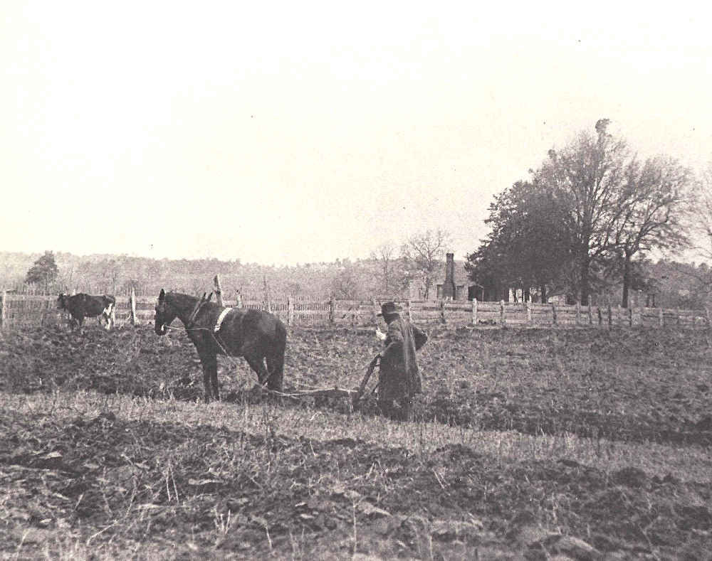
Farmers producing commodities: price takers, no market power.
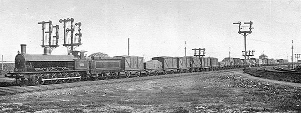
Railroads transporting goods:
price setters, lots of market power.
"Market Power" doesn't actually require a monopoly
Competition
- Lots of "small" firms selling basically the same thing
Market Power
- One or a few "medium" or "large" firms selling differentiated products
- Firms face essentially horizontal demand curve
- Firms face downward sloping demand curve
Monopoly as Metaphor
- True "monopolies" are rare
- Firms with some (at least local) market power are common
- We'll use "monopoly" as a metaphor
to analyze any firm that doesn't take prices as given,
and therefore faces a downward-sloping demand curve.
Review: Revenue, Marginal Revenue, and Elasticity
Demand and Inverse Demand
Demand curve:
quantity as a function of price
Inverse demand curve:
price as a function of quantity
QUANTITY
PRICE
If the firm wants to sell \(q\) units, it sells all units at the same price \(p(q)\)
Since all units are sold for \(p\), the average revenue per unit is just \(p\).
By the product rule...
let's delve into this...
Total, Average, and Marginal Revenue
The total revenue is the price times quantity (area of the rectangle)
Note: \(MR < 0\) if
The total revenue is the price times quantity (area of the rectangle)
If the firm wants to sell \(dq\) more units, it needs to drop its price by \(dp\)
Revenue loss from lower price on existing sales of \(q\): \(dp \times q\)
Revenue gain from additional sales at \(p\): \(dq \times p\)
Marginal Revenue and Elasticity
(multiply first term by \(p/p\))
(simplify)
(since \(\epsilon < 0\))
Notes
Elastic demand: \(MR > 0\)
Inelastic demand: \(MR < 0\)
In general: the more elastic demand is, the less one needs to lower ones price to sell more goods, so the closer \(MR\) is to \(p\).
Profit Maximization with Market Power
Optimize by taking derivative and setting equal to zero:
Profit is total revenue minus total costs:
"Marginal revenue equals marginal cost"
Example:
What is the profit-maximizing value of \(q\)?
What is the profit-maximizing value of \(q\)?
Multiply right-hand side by \(q/q\):
Profit is total revenue minus total costs:
"Profit per unit times number of units"
AVERAGE PROFIT
CHECK YOUR UNDERSTANDING
Find the profit-maximizing quantity.

Elasticity and Profit Maximization
Recall our elasticity representation of marginal revenue:
Let's combine it with this
profit maximization condition:
Really useful if MC and elasticity are both constant!
Inverse elasticity pricing rule:
Find the optimal price and quantity if a firm has the cost function $$c(q) = 200 + 4q$$ and faces the demand curve $$D(p) = 6400p^{-2}$$
Inverse elasticity pricing rule:
One more way of slicing it...
Fraction of price that's markup over marginal cost
(Lerner Index)
What if \(|\epsilon| \rightarrow \infty\)?