Demand
Christopher Makler
Stanford University Department of Economics
Econ 50: Lecture 11
Today's Agenda
Part 1:
Comparative Statics
Part 2:
Functional Forms and Behavior
- Changes in price:
- Price offer curves
- Demand curves
- Complements and Substitutes
- Changes in income:
- Income offer curves
- Engel curves
- Normal, and inferior goods
- Cobb-Douglas
- Perfect Complements
- Perfect Substitutes
- Quasilinear
Last Two Classes: What is the optimal bundle for a given budget line?
Today: What happens to the optimal bundle when prices/income change?
🍏
🍌
BL1
We will be solving for the optimal bundle
as a function of income and prices:
The solutions to this problem will be called the demand functions. We have to think about how the optimal bundle will change when \(p_1,p_2,m\) change.
BL2
Specific Prices & Income
General Prices & Income
Plug tangency condition back into constraint:
Tangency Condition: \(MRS = p_1/p_2\)
Specific Prices & Income
General Prices & Income
OPTIMAL BUNDLE
DEMAND FUNCTIONS
(optimization)
(comparative statics)
Remember what you learned about demand and demand curves in Econ 1 / high school:
- The demand curve shows the quantity demanded of a good at different prices
- A change in the price of a good results in a movement along its demand curve
- A change in income or the price of other goods results in a shift of the demand curve
-
- If two goods are substitutes, an increase in the price of one will increase the demand for the other (shift the demand curve to the right).
- If two goods are complements, an increase in the price of one will decrease the demand for the other (shift the demand curve to the left).
- If a good is a normal good, an increase in income will increase demand for the good
- If a good is an inferior good, an increase in income will decrease demand the good
Three Relationships
...its own price changes?
Movement along the demand curve
...the price of another good changes?
Complements
Substitutes
Independent Goods
How does the quantity demanded of a good change when...
...income changes?
Normal goods
Inferior goods
Giffen goods
(possible) shift of the demand curve
Three Relationships
...its own price changes?
Movement along the demand curve
How does the quantity demanded of a good change when...
The demand curve for a good
shows the quantity demanded of that good
as a function of its own price
holding all other factors constant
(ceteris paribus)
The price offer curve shows how the optimal bundle changes in good 1-good 2 space as the price of one good changes.
DEMAND CURVE FOR GOOD 1
"Good 1 - Good 2 Space"
"Quantity-Price Space for Good 1"
PRICE OFFER CURVE
Three Relationships
...the price of another good changes?
How does the quantity demanded of a good change when...
Substitutes
Complements
When the price of one good goes up, demand for the other increases.
When the price of one good goes up, demand for the other decreases.


Independent
Demand not related
Complements: \(p_2 \uparrow \Rightarrow x_1^* \downarrow\)
What happens to the quantity of good 1 demanded when the price of good 2 increases?
Substitutes: \(p_2 \uparrow \Rightarrow x_1^* \uparrow\)
COMPLEMENTS:
UPWARD-SLOPING
PRICE OFFER CURVE
SUBSTITUTES:
DOWNWARD-SLOPING
PRICE OFFER CURVE
Three Relationships
How does the quantity demanded of a good change when...
...income changes?
Normal Goods
Inferior Goods
When your income goes up,
demand for the good increases.
When your income goes up,
demand for the good decreases.

The income offer curve shows how the optimal bundle changes in good 1-good 2 space as income changes.
Good 1 normal: \(m \uparrow \Rightarrow x_1^* \uparrow\)
What happens to the quantity of good 1 demanded when the income increases?
Good 1 inferior: \(m \uparrow \Rightarrow x_1^* \downarrow\)
BOTH NORMAL GOODS:
UPWARD-SLOPING
INCOME OFFER CURVE
ONE GOOD INFERIOR:
DOWNWARD-SLOPING
PRICE OFFER CURVE
- A change in the price of a good results in a movement along its demand curve
- A change in income or the price of other goods results in a shift of the demand curve
Things to Think About
Think about how the behavior described by the demand function translates into the overall shape of the demand curve:
- Are there discontinuities/cutoff prices where behavior changes?
- What happens as the price gets really high, or approaches zero?
- What fraction of income is being spent on this good?
The reason we use different utility functions is because people's relationship with prices depends on the nature of their preferences.
Note: Maximum Possible Quantity Demanded

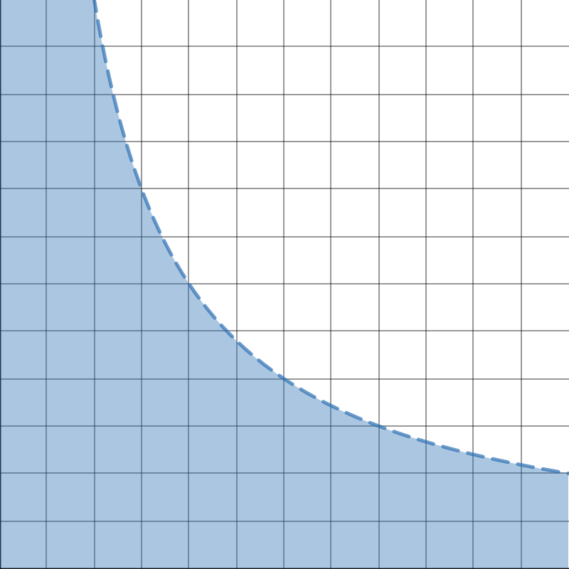
Quantity of Good 1 \((x_1)\)
Price of Good 1 \((p_1)\)
All demand curves must be in this region
Quantity bought at each price if you spent all your money on good 1