Production and Cost
for a Firm
Christopher Makler
Stanford University Department of Economics
Econ 50 : Lecture 16
Today's Agenda
- Overview of Unit III
- Review of Econ 1 Treatment of Production and Cost
- Total, Marginal, and Average Costs
- Short-Run and Long-Run Costs
- Curvature of Cost Functions
Unit I: The “Real Economy"
Labor
Fish
🐟
Capital
Coconuts
🥥
[GOODS]
⏳
⛏
[RESOURCES]
Utility
🤓
The story thus far...
Unit II: Consumers and Prices
Labor
Fish
🐟
Capital
Coconuts
🥥
[GOODS]
⏳
⛏
[RESOURCES]
🤓
Consumer
The story thus far...
Unit III: Theory of the Firm
Labor
Firm
🏭
Capital
⏳
⛏
Customers
🤓
This unit: analyze the firms
consumers buy things from
Unit III: Theory of the Firm
Firm
🏭
Costs
Customers
🤓
This unit: analyze the firms
consumers buy things from
Unit III: Theory of the Firm
Firm
🏭
Costs
Revenue
From the firm's perspective, they get revenue and pay costs...
Unit III: Theory of the Firm
Costs
Revenue
Profit
...which is what we call profits
Unit III: Theory of the Firm
Costs
Revenue
Profit
Today: determine the firm's cost as a function of \(q\)
Wednesday: determine the firm's revenue as a function of \(q\)
Friday: find the firm's profit-maximizing value of \(q\)
Unit III: Theory of the Firm
How much output \(q\) does it supply as a function of the price of the good?
How much labor \(L\) does it demand as a function of the wage rate?
Next week: analyze the behavior of a competitive (price-taking) firm
The Econ 1 Approach
Greg Mankiw, Principles of Economics
Greg Mankiw, Principles of Economics
Greg Mankiw, Principles of Economics
Greg Mankiw, Principles of Economics
Greg Mankiw, Principles of Economics
Dollars
Dollars Per Unit
The Econ 50 Approach
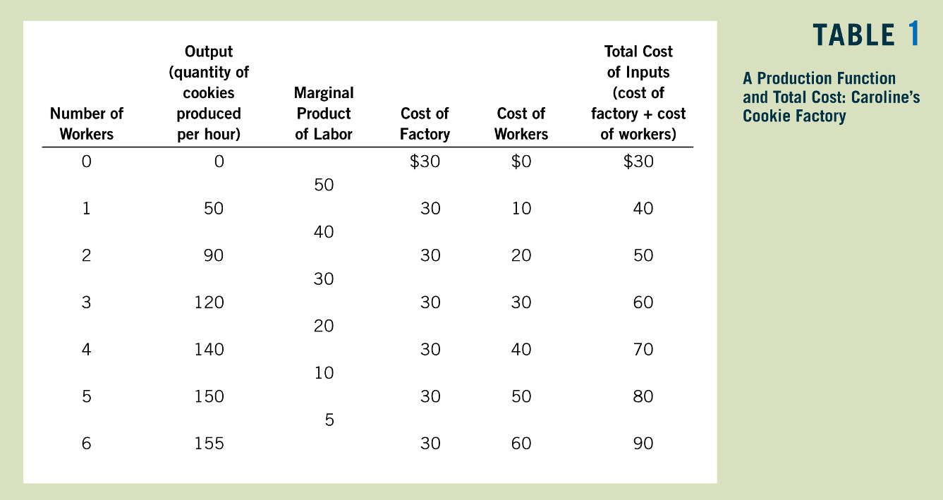
Let's start with just one input, labor, so \(q = f(L)\)
The total cost will be the cost of that labor input:
Just as with the PPF, we can talk about the labor required to produce \(q\) units of output, \(L(q)\)
\(TC(q) = wL(q)\)
\(TC(q) = wL(q)\)
Now, let's add capital.
We will assume that the level of capital is fixed in the short run at some amount \(\overline K\).
The amount of labor required to produce \(q\) units of output is therefore also going to depend upon \(\overline K\):
Short-Run Total Cost of \(q\) Units
Variable cost
"The total cost of producing \(q\) units in the short run is the variable cost of the required amount of the input that can be varied,
plus the fixed cost of the input that is fixed in the short run."
Fixed cost
Short-run conditional demand for labor
if capital is fixed at \(\overline K\):
Total cost of producing \(q\) units of output:
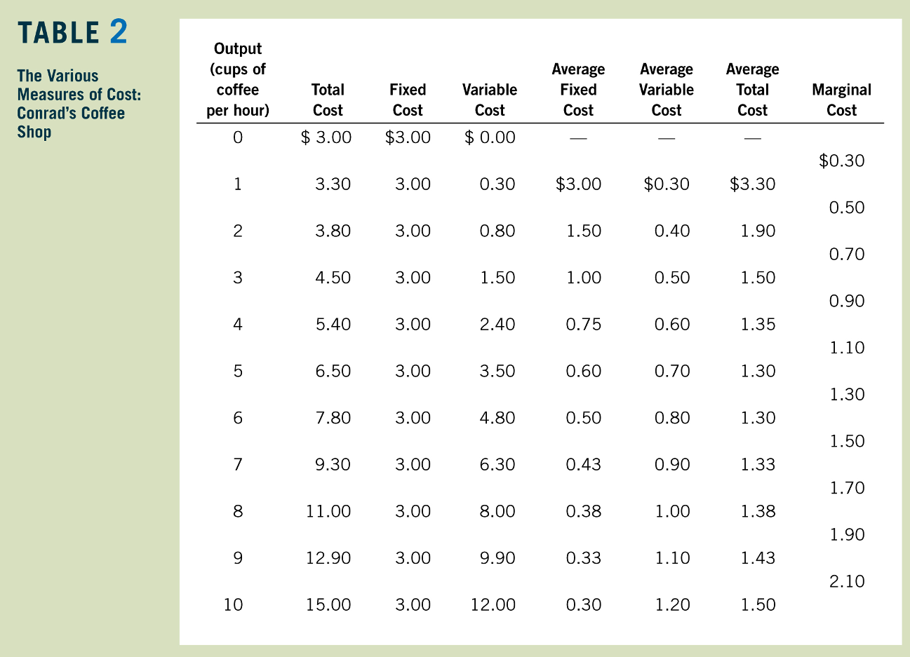
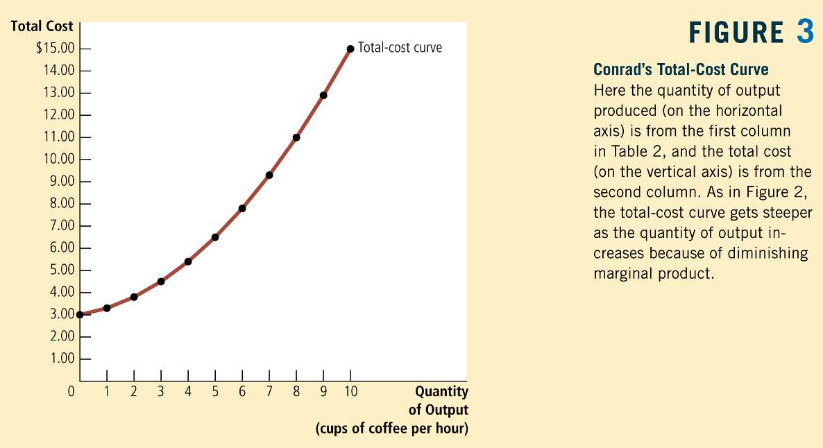
Total, Fixed and Variable Costs
Fixed Costs \((F)\): All economic costs
that don't vary with output.
Variable Costs \((VC(q))\): All economic costs
that vary with output
explicit costs (\(r \overline K\)) plus
implicit costs like opportunity costs
e.g. cost of labor required to produce
\(q\) units of output given \(\overline K\) units of capital
pollev.com/chrismakler

Generally speaking, if capital is fixed in the short run, then higher levels of capital are associated with _______ fixed costs and _______ variable costs for any particular target output.
Fixed Costs
Variable Costs
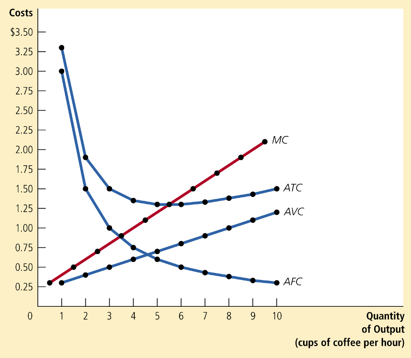
Average Fixed Costs (AFC)
Average Variable Costs (AVC)
Average Costs
Average Costs
Fixed Costs
Variable Costs
Marginal Cost
(marginal cost is the marginal variable cost)
Marginal Cost
pollev.com/chrismakler
Suppose q* is the quantity
for which ATC is lowest.
Which of the following must be true?
(Assume that ATC and MC are continuous functions of q.)
(a) MC also reaches its minimum at q*
(b) MC reaches its maximum at q*
(c) MC and ATC are equal at q*
Marginal cost tends to "pull" average cost toward it:
Marginal grade = grade on last test, average grade = GPA
Relationship between Average and Marginal Costs
Relationship between Marginal Cost and Marginal Product of Labor
Next Time
- Think about the demand curve facing a firm
- Analyze the price elasticity of demand
- Analyze the total and marginal revenue from producing more output
- Friday: bring cost and revenue together
Cost Minimization
Cost Minimization Subject to a Utility Constraint
Cost Minimization Subject to an Output Constraint
Hicksian Demand
Conditional Demand
Cost Minimization: Lagrange Method
First Order Conditions
MRTS (slope of isoquant) is equal to the price ratio
Tangency condition: \(MRTS = w/r\)
Constraint: \(q = f(L,K)\)
Conditional demands for labor and capital:
Total cost of producing \(q\) units of output:
Expansion Path
A graph connecting the input combinations a firm would use as it expands production: i.e., the solution to the cost minimization problem for various levels of output
Exactly the same as the income offer curve (IOC) in consumer theory.
(And, if the optimum is found via a tangency condition, exactly the same as the tangency condition.)
Long-Run Total Cost of \(q\) Units
Conditional demand for labor
Conditional demand for capital
"The total cost of producing \(q\) units in the long run
is the cost of the cost-minimizing combination of inputs
that can produce \(q\) units of output."
Exactly the same as the expenditure function in consumer theory.
Long Run (can vary both labor and capital)
Short Run with Capital Fixed at \(\overline K \)
Long Run (can vary both labor and capital)
Short Run with Capital Fixed at \(\overline K \)
Let's fix \(w= 8\), \(r = 2\), and \(\overline K =32\)
Relationship between
Short-Run and Long-Run Costs
What conclusions can we draw from this?
Returns to a Single Input
- Increasing marginal product: MPL is increasing in L
- Constant marginal product: MPL is constant in L
- Diminishing marginal product: MPL is decreasing in L
Returns to Scale (Scaling all inputs.)
- Increasing returns to scale: doubling all inputs more than doubles output.
- Constant returns to scale: doubling all inputs exactly doubles output.
- Decreasing returns to scale: doubling all inputs less than doubles output.
Relationship between Production Function and the Curvature of Long-Run and Short-Run Costs
- If the production function has diminishing \(MP_L\), the short-run cost curve will get steeper as you produce more output
- If the production function has decreasing returns to scale, the long-run cost curve will get steeper as you produce more output.
- What about for constant returns to scale? Increasing returns to scale?
- Homework question 15.1 walks you through these...
Economies and Diseconomies of Scale
Returns to Scale
Has to do with the production function
Economies of Scale
Has to do with cost curves
Increasing Returns to Scale:
double input => more than double output
Decreasing Returns to Scale:
double input => less than double output
Always deals with the long run
Can occur in both the long run and short run
Economies of Scale:
increasing output lowers average costs
Diseconomies of Scale:
increasing output raises average costs