Market Power
Christopher Makler
Stanford University Department of Economics
Econ 50 : Lecture 24
pollev.com/chrismakler

Name a company.
Today's Agenda
- Why profits should approach zero
if markets are competitive - Why firms can persistently run profits in real life
if firms have market power - The effect of increased consolidation
- The welfare effect of market power
- Monopsony: market power in input markets
The "Zero Profit Condition"
Profits in industry 1 when profit maximizing
Profits in industry 2 when profit maximizing
A firm in industry 1 should remain in industry 1 as long as
"Positive economic profit"
SR fixed costs
LR fixed costs
The Effect of Entry and Exit
Industry Short Run:
Number of Firms is Fixed
Industry Long Run:
Firms will enter an industry with positive economic profits; firms will leave an industry with negative economic profits.
In long-run competitive equilibrium, firms in all industries make nonnegative economic profit.
Definition: Minimum Efficient Scale
A firm's minimum efficient scale (MES) is the quantity at which average cost is the lowest.
If MC is increasing, this coincides with the quantity at which MC = AC.
Market Supply and Demand
Typical Firm's Cost Curves
MC
y
$ perunit
P
Q
S
1. demand
increases
D'
D
AC
What is the effect of an increase in demand?
S'
3. firms
enter
\(S_{LR}\)
How to Solve for Long-Run Equilibrium
- Find marginal cost function, \(MC(q) = c'(q)\).
- Set \(p = MC(q)\) and solve for the individual firm supply function, \(q^*(p)\).
- Multiply \(q^*(p)\) by the number of firms \(N_F\) to get the market supply curve \(S(p, N_F)\).
- Set \(D(p) = S(p,N_F)\) and solve for \(p\) to find the equilibrium market price as a function of \(N_F\)
Part I: Solve for the short-run equilibrium price as a function of the number of firms.
Part II: Find the long-run equilibrium price and solve for the equilibrium number of firms.
- Find the average cost function, \(AC(q) = c(q)/q\).
- Set \(AC(q) = MC(q)\) and solve for the minimum efficient scale (MES).
- The LR price is the MC and AC at the MES; plug this into step 4 above and solve for \(N_F\)!
Most important takeaways
Firms optimize by setting MR = MC
Entry and exit forces AR = AC
pollev.com/chrismakler
What does the equals sign in the condition
\(AR = AC\) represent?
The Real World
The world is not perfectly competitive.

Market in LR Equilibrium
(profits equal
across industries)
Increased demand
Higher prices
Higher profits in this industry than others
(exogenous shock)
New firms enter
Increased supply
Lower prices
(self-regulating mechanism)
...but what happens if there are barriers to entry?
Market in LR Equilibrium
(profits equal
across industries)
Increased demand
Higher prices
Higher profits in this industry than others
(exogenous shock)
New firms enter
Increased supply
Lower prices
BARRIERS TO ENTRY


"It is better to buy than compete" - Mark Zuckerberg
Markups
The total revenue is the price times quantity (area of the rectangle)
Note: \(MR < 0\) if
The total revenue is the price times quantity (area of the rectangle)
If the firm wants to sell \(dq\) more units, it needs to drop its price by \(dp\)
Revenue loss from lower price on existing sales of \(q\): \(dp \times q\)
Revenue gain from additional sales at \(p\): \(dq \times p\)
Marginal Revenue and Elasticity
(multiply first term by \(p/p\))
(definition of elasticity)
(since \(\epsilon < 0\))
Notes
Elastic demand: \(MR > 0\)
Inelastic demand: \(MR < 0\)
In general: the more elastic demand is, the less one needs to lower ones price to sell more goods, so the closer \(MR\) is to \(p\).
We've just derived an elasticity
representation of marginal revenue:
Let's combine it with this
profit maximization condition:
Really useful if MC and elasticity are both constant!
Inverse elasticity pricing rule:
One more way of slicing it...
Fraction of price that's markup over marginal cost
(Lerner Index)
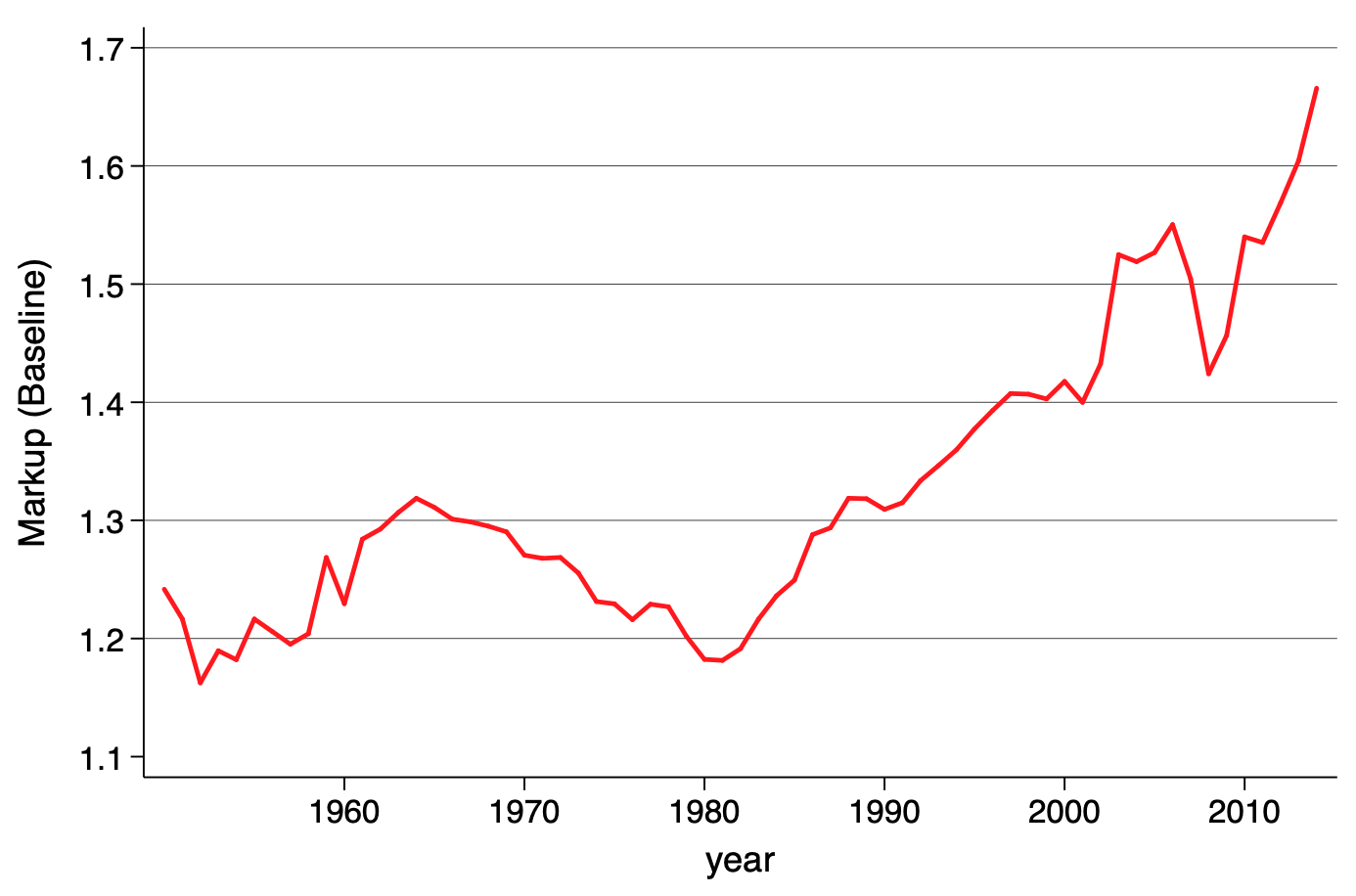
De Loecker & Eeckhout (QJE 2020)
Welfare Effects
Monopsony
Profit as a function of output \(q\)
Profit as a function of labor \(L\)
1. Costs for general \(w\) and revenue for general \(p\)
2. Profit = total revenues minus total costs
3. Take derivative of profit function, set =0
PROFIT-MAXIMIZING OUTPUT SUPPLY
PROFIT-MAXIMIZING LABOR DEMAND
Profit as a function of output \(q\)
Profit as a function of labor \(L\)
1. Costs for general \(w\) and revenue for general \(p\)
2. Profit = total revenues minus total costs
3. Take derivative of profit function, set =0
[cost of labor required for \(q\) units of output]
[revenue of output produced by \(L\) hours of labor]
MARGINAL COST (MC)
MARGINAL REVENUE PRODUCT OF LABOR (MRPL)
"Keep producing output as long as the marginal revenue from the last unit produced is at least as great as the marginal cost of producing it."
"Keep hiring workers as long as the marginal revenue from the output of the last worker is at least as great as the cost of hiring them."
Profit as a function of output \(q\)
Profit as a function of labor \(L\)
Monopsony: the firm has market power in labor markets.
Suppose a monopsonist faces a labor supply curve given by
What wage rate would it need to set if it wanted to hire 60 workers?
pollev.com/chrismakler
What would the total cost of hiring 60 workers be?
What would the marginal cost of hiring a 61st worker be?
Monopsony: the firm has market power in labor markets.
Suppose a monopsonist faces a labor supply curve given by
If it wanted to hire \(L\) workers, it would need to set wage
The total cost of hiring \(L\) workers would be
The marginal cost of hiring another worker is
Monopsony vs. Monopoly
- Firms with market power in output markets keep production low to keep prices high.
- Firms with market power in input markets keep their labor force low to keep wages low
- Firms that are both are bad for both workers and consumers

Next Time
- Review of Econ 50
- Preview of Econ 51