Course Retrospective
Christopher Makler
Stanford University Department of Economics
Econ 50: Lecture 25

Ways to Think about Learning
Strategic:
"knowing when" - given an unstructured problem, which model/framework is most relevant?
Schematic:
Procedural:
Declarative:
"knowing why" - how do different concepts/models relate to one other?
"knowing how" - given a well-defined problem, ability to follow correct procedure to solve it
"knowing that" - facts and figures, vocabulary
Goals of the Course
Strategic:
Develop rigorous approach to economic modeling; understand how assumptions map into conclusions.
Schematic:
Procedural:
Declarative:
Understand the relationships between
words, math, and graphs.
Learn the techniques of
optimization, equilibrium, and comparative statics.
Know the definitions of key economic terms.
Two Kinds of Optimization
Tradeoffs between two goods
Optimal quantity of one good
🍎
(not feasible)
(feasible)
🍌
Optimal choice
🙂
😀
😁
😢
🙁
🍎
benefit and cost per unit
Marginal Cost
Marginal Benefit
Optimal choice
Tradeoffs between two goods
Optimal quantity of one good
Checkpoint 1: October 13
Model 1: Consumer Choice
Model 2: Theory of the Firm
Checkpoint 2: October 27
WEEK 1
WEEK 2
WEEK 3
Modeling preferences with multivariable calculus
Constrained optimization when calculus works
Constrained optimization when calculus doesn't work
WEEK 4
WEEK 5
Consumer Demand
Applications to Finance
Checkpoint 3: November 10
Final Exam: December 12 (cumulative)
WEEK 6
WEEK 7
WEEK 8
Production and Costs for a Firm
Profit Maximization
Competitive Equilibrium
WEEK 9
WEEK 10
Taxes and Externalities
Public Economics; Market Power
Model 3: Market Equilibrium
Today's Agenda
- Optimization
- Preferences and Utility
- Optimization subject to a budget constraint
- Comparative Statics
- Consumer demand
- Firm supply
- Equilibrium
- When markets work
- When markets need tweaking
- When markets fail
Today's Agenda
- Optimization
- Preferences and Utility
- Optimization subject to a budget constraint
- Comparative Statics
- Consumer demand
- Firm supply
- Equilibrium
- When markets work
- When markets need tweaking
- When markets fail
First half of the class:
Analyzing tradeoffs
Choices in general
Choices of commodity bundles
Choosing bundles of two goods
Good 1 \((x_1)\)
Good 2 \((x_2)\)
Completeness axiom:
any two bundles can be compared.
Implication: given any bundle \(A\),
the choice space may be divided
into three regions:
preferred to A
dispreferred to A
indifferent to A
Indifference curves cannot cross!
A
The indifference curve through A connects all the bundles indifferent to A.
Indifference curve
through A
Special Case: Good 1 - Good 2 Space
Marginal Rate of Substitution
🍏🍏
🍏🍏
🍏🍏
🍏🍏
🍏🍏
🍌🍌🍌🍌
🍌🍌🍌🍌
🍌🍌🍌🍌
🍌🍌🍌🍌
🍌🍌🍌🍌
🍌🍌🍌🍌
🍏🍏
🍏🍏
🍏🍏
🍏🍏
🍏🍏
🍏🍏
🍌🍌🍌🍌
🍌🍌🍌🍌
🍌🍌🍌🍌
🍌🍌🍌🍌
🍌🍌🍌🍌
Suppose you were indifferent between the following two bundles:
Starting at bundle X,
you would be willing
to give up 4 bananas
to get 2 apples
Let apples be good 1, and bananas be good 2.
Starting at bundle Y,
you would be willing
to give up 2 apples
to get 4 bananas
Visually: the MRS is the magnitude of the slope
of an indifference curve
Calculating the MRS
Along an indifference curve, all bundles will produce the same amount of utility
In other words, each indifference curve
is a level set of the utility function.
The slope of an indifference curve is the MRS. By the implicit function theorem,
UTILS
UNITS OF GOOD 1
UTILS
UNITS OF GOOD 2
Intertemporal choice: \(c_1\), \(c_2\) represent
consumption in different time periods.
Risk aversion: \(c_1\), \(c_2\) represent
consumption in different states of the world.
Applications: Foundations of Finance
If \(v(c)\) exhibits diminishing marginal utility:
MRS is higher if you have less money today
and/or more money tomorrow
MRS is lower if you are more patient (\(\beta\) is high)
MRS is higher if state 1 is more likely to occur
(\(\pi\) is higher)
Let \(v(c)\) be the value function describing how much utility you get from money/consumption
Desirable Properties of Preferences
We've asserted that all (rational) preferences are complete and transitive.
There are some additional properties which are true of some preferences:
- Monotonicity
- Convexity
- Continuity
- Smoothness
Monotonic Preferences: “More is Better"
Convex Preferences: “Variety is Better"
Take any two bundles, \(A\) and \(B\), between which you are indifferent.
Would you rather have a convex combination of those two bundles,
than have either of those bundles themselves?
If you would always answer yes, your preferences are convex.
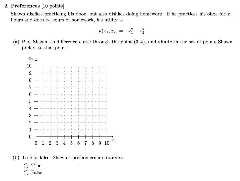
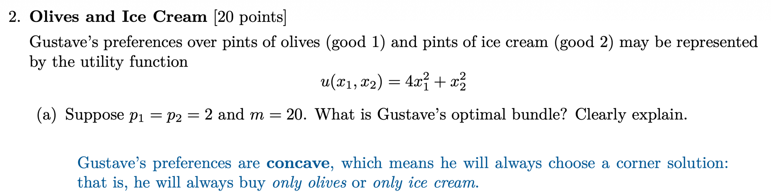
Concave Preferences: “Variety is Worse"
Take any two bundles, \(A\) and \(B\), between which you are indifferent.
Would you rather have a convex combination of those two bundles,
than have either of those bundles themselves?
If you would always answer no, your preferences are concave.

Modeling preferences with functional forms


Perfect Substitutes
Goods that can always be exchanged at a constant rate.
-
Red pencils and blue pencils, if you con't care about color
-
One-dollar bills and five-dollar bills
-
One-liter bottles of soda and two-liter bottles of soda
Cobb-Douglas
An easy mathematical form with interesting properties.
-
Used for two independent goods (neither complements nor substitutes) -- e.g., t-shirts vs hamburgers
-
Also called "constant shares" for reasons we'll see later.
Normalizing Cobb-Douglas Functions
One reason to transform a utility function is to normalize it.
This allows us to describe preferences using fewer parameters.
[ multiply by \({1 \over a + b}\) ]
[ let \(\alpha = {a \over a + b}\) ]
Normalizing Cobb-Douglas Functions
One reason to transform a utility function is to normalize it.
This allows us to describe preferences using fewer parameters.
[ raise to the power of \({1 \over a + b}\) ]
[ let \(\alpha = {a \over a + b}\) ]
pollev.com/chrismakler
The utility function
represents the same preferences as the utility function
for what value of \(\alpha\)?
Preferences over Time
Examples:
Preferences over Risk
pollev.com/chrismakler
If you are risk loving, what does that say about your preferences over consumption in different states of the world?
Today's Agenda
- Optimization
- Preferences and Utility
- Optimization subject to a budget constraint
- Comparative Statics
- Consumer demand
- Firm supply
- Equilibrium
- When markets work
- When markets need tweaking
- When markets fail
Choice space:
all possible options
Feasible set:
all options available to you
Optimal choice:
Your best choice(s) of the ones available to you
Constrained Optimization
One type of feasible set: the budget set
Endowment Budget Line
Good 1
Good 2
pollev.com/chrismakler
You have some apples (good 1) and oranges (good 2).
You can sell some of one and use the proceeds to buy the other.
If the price of apples (good 1) increases, how does this impact the intercepts of your budget line?
Kinked Constraints
- Remember: the slope of the budget line is the price ratio (opportunity cost of good 1)
- Straight budget line: every unit of every good costs the same amount
- Kinked budget constraint: prices of at least one good are different over different portions of the constraint
Different Prices for Buying and Selling
Tickets
Money
If you sell all your tickets,
how much money will you have?
If you spend all your money on additional tickets, how many tickets will you have?
Suppose you have 40 tickets and $1200.
1200
40
2200
Slope = \(p^{\text{sell}}\) = $25/ticket
Slope = \(p^{\text{buy}}\) = $60/ticket
You can sell tickets for $25 each,
or buy additional tickets for $60 each.
60
Intertemporal Budget Line
All of these budget lines had different stories, but they're fundamentally the same thing:
they all divide the choice space
into affordable and unaffordable bundles.
Combining preferences and constraints
IF...
THEN...
The consumer's preferences are "well behaved"
-- smooth, strictly convex, and strictly monotonic
\(MRS=0\) along the horizontal axis (\(x_2 = 0\))
The budget line is a simple straight line
The optimal consumption bundle will be characterized by two equations:
More generally: the optimal bundle may be found using the Lagrange method
\(MRS \rightarrow \infty\) along the vertical axis (\(x_1 \rightarrow 0\))
The Lagrange Method
Cost of Bundle X
Income
Utility
The Lagrange Method
Income left over
Utility
The Lagrange Method
Income left over
Utility
(utils)
(dollars)
utils/dollar
First Order Conditions
"Bang for your buck" condition: marginal utility from last dollar spent on every good must be the same!
The Lagrange Method
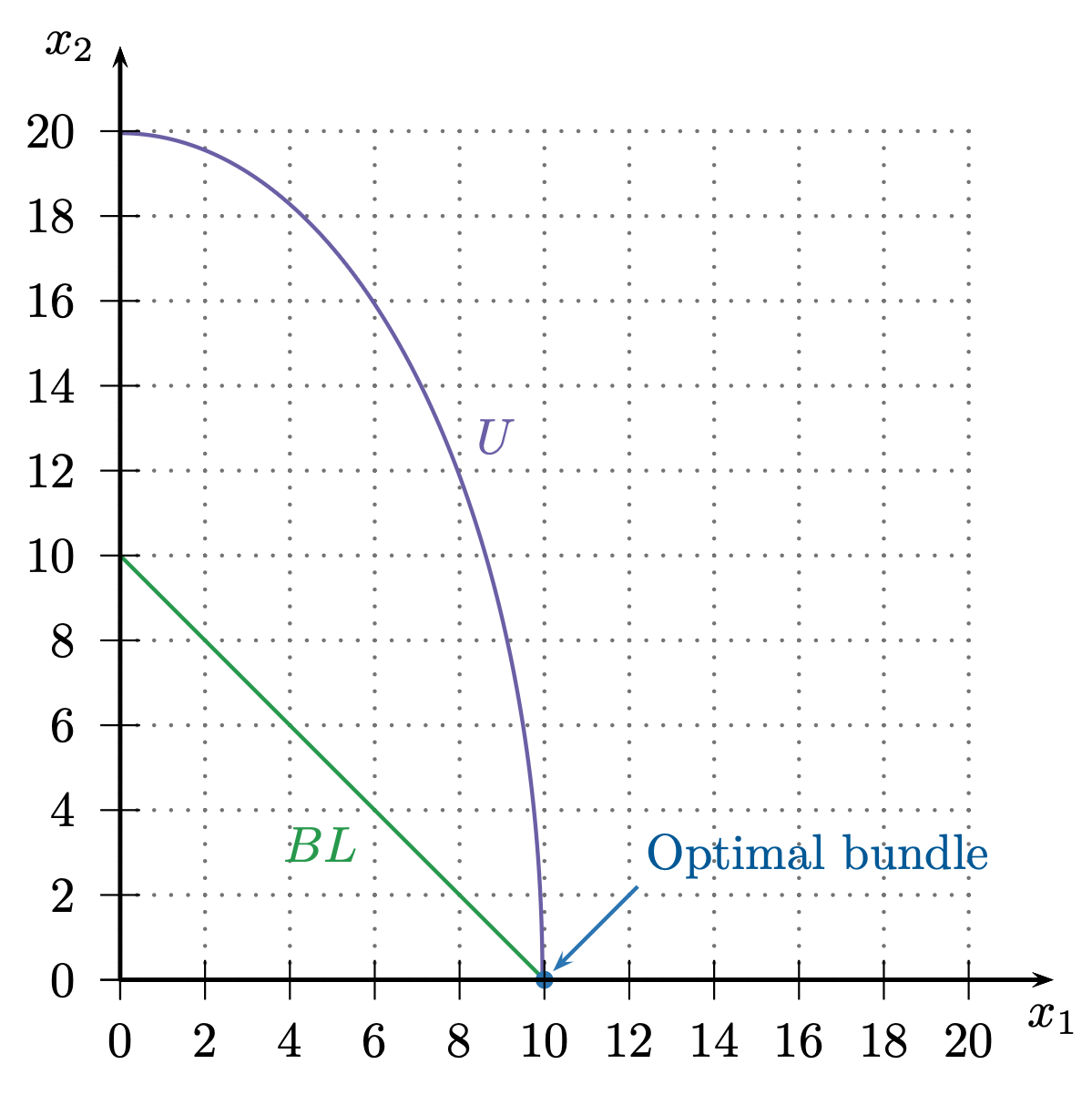
What happens when the Lagrange method fails?
- Corner solutions
- Solutions at kinks
Interior Solution:
Corner Solution:
Optimal bundle contains
strictly positive quantities of both goods
Optimal bundle contains zero of one good
(spend all resources on the other)
If only consume good 1: \(MRS \ge {p_1 \over p_2}\) at optimum
If only consume good 2: \(MRS \le {p_1 \over p_2}\) at optimum
Corner Solutions
\(MRS < {p_1 \over p_2}\) along
the entire budget line!
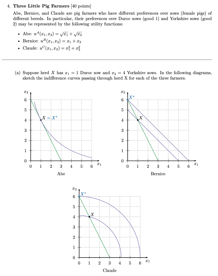
For which of the three farmers did the Lagrange method find the optimal bundle?
(Note: this is the 50 version;
the 50Q version reversed Abe and Claude.)
Summary: Constrained Optimization
- Analysis of tradeoffs
- Lagrange multiplier represents the "exchange rate" between the units of the objective function and the units of the constraint.
- Lagrange method works by equating "bang for your buck" across competing goods.
- However, some solutions occur at corners or kinks where bang for your buck is not equated; in that case, have to apply logic.
Today's Agenda
- Optimization
- Preferences and Utility
- Optimization subject to a budget constraint
- Comparative Statics
- Consumer demand
- Firm supply
- Equilibrium
- When markets work
- When markets need tweaking
- When markets fail
Optimization: What is the optimal bundle for a given situation?
Comparative Statics: What happens to the optimal bundle when something about that situation changes?
🍏
🍌
BL1
Example: solve for the optimal bundle
as a function of income and prices:
The solutions to this problem will be called the demand functions. We have to think about how the optimal bundle will change when \(p_1,p_2,m\) change.
BL2
Based on this, what must Gustave's demand curve look like?
- A change in the price of a good results in a movement along its demand curve
- A change in income or the price of other goods results in a shift of the demand curve
Today's Agenda
-
Optimization
- Preferences and Utility
- Optimization subject to a budget constraint
- Comparative Statics
- Consumer demand
- Firm supply
- Equilibrium
- When markets work
- When markets need tweaking
- When markets fail
Relationship between Marginal Cost and Marginal Product of Labor
Perfectly Inelastic
Inelastic
Unit Elastic
Elastic
Perfectly Elastic
Doesn't change
Changes by less than the change in X
Changes proportionally to the change in X
Changes by more than the change in X
Changes "infinitely" (usually: to/from zero)
How does the endogenous variable Y respond to a
change in the exogenous variable X?
(note: all of these refer to the ratio of the perentage change, not absolute change)
The more elastic demand is, the less MR is different than price.
We've just derived an elasticity
representation of marginal revenue:
Let's combine it with this
profit maximization condition:
Really useful if MC and elasticity are both constant!
Inverse elasticity pricing rule:
If a firm has the cost function $$c(q) = 200 + 4q$$ and faces the demand curve $$D(p) = 6400p^{-2}$$ what is its optimal price?
Inverse elasticity pricing rule:
Marginal Revenue for Perfectly Elastic Demand
(multiply first term by \(p/p\))
(simplify)
(since \(\epsilon < 0\))
Note
Perfectly elastic demand: \(MR = p\)
Price
MC
\(q\)
$/unit
P = MR
12
24
Analyzing Comparative Statics
- Solve the optimization problem as a function of the variables that will shift the solution
- Try to determine if there are key points where behavior changes
- Know how to tell a story with a graph: most times, you don't have to graph things precisely, just show how a change percolates graphically through a model!
Today's Agenda
-
Optimization
- Preferences and Utility
- Optimization subject to a budget constraint
-
Comparative Statics
- Consumer demand
- Firm supply
-
Equilibrium
- When markets work
- When markets need tweaking
- When markets fail
Important Note: Three Kinds of “=" Signs
1. Mathematical Identity: holds by definition
2. Optimization condition: holds when an agent is optimizing
3. Equilibrium condition: holds when a system is in equilibrium
WEEK 8
Partial Equilibrium
WEEK 9
WEEK 10
Taxes and Externalities
Public Goods and Common Resources
Market Power
Lecture 19: What price and quantity will the market determine?
Lecture 20: The market will maximize total welfare by equating MB = MC.
Lecture 21: Taxes generate deadweight loss because they get in the way of people setting MB = MC.
Lecture 22: In the presence of externalities, agents don't face their true MB or MC; taxes can correct this.
Lecture 23: There are some kinds of goods for which the market will never work, because (private) MB/MC is not well defined.
Lecture 24: Firms with market power don't set their MC equal to consumers' MB; model of competitive markets doesn't apply.
MARKETS ARE GREAT! 😇
MARKETS NEED MINOR TWEAKS 😕
MARKETS WON'T SAVE US 😭
Pigovian tax:
Internalize the externality so that private marginal cost equals social marginal cost.
Competitive equilibrium:
consumers set \(P = MB\),
producers set \(P = PMC \Rightarrow MB = PMC\)
With a tax: consumers set \(P = MB\),
producers set \(P - t = PMC\)
Fees
Suppose you needed to buy a fishing permit for a fee F.
What value of F would result in the optimal L*?
Taxes
Suppose the village levied a tax of t per fish caught.
What value of t would result in the optimal L*?
What do I want you to take away from this?
- Not the details: your boss will literally never ask you to set up a Lagrangian, and they won't know what the heck Kuhn-Tucker is.
- At the core of every model are people making choices.
- The first step to creating a model is figuring out what people want: preferences/utility, profit, etc.
- The next step is figuring out what constraints they're operating under, and how they would respond to changes in those constraints.
- Finally, you want to model what happens when those people (and firms, and governments) interact with one another.
- Our analysis of that has been pretty basic: people interact with each other only in markets, where they're all anonymous price takers...


Model 1: Trading
Model 3: Strategic Interactions
with Incomplete Information
WEEK 1
WEEK 2
WEEK 3
Preferences
Exchange Economies
Production Economies
WEEK 4
WEEK 5
Analyzing a Game from a Player's POV
Static Games of Complete Information
WEEK 6
WEEK 7
WEEK 8
Dynamic Games of Complete Information
Static Games of Incomplete Information
Dynamic Games of Incomplete Information
WEEK 9
WEEK 10
Getting people to do what you want
Getting people to reveal information
Model 4: Interactions with Asymmetric Information
Econ 51: All about different types of interactions
Model 2: Strategic Interactions with Complete Information
But for now...preparing for the exam
- Relatively few mathematical techniques
- Lots of different applications
- Within each application, know your definitions well so you can apply the relevant techniques.
- Read the questions carefully, think before you write, and don't do too much work: most questions can be answered without solving for an optimum.
- Good luck!