Welcome To Econ 51
Part 2: Review of Consumer Theory
Econ 51, Lecture 1
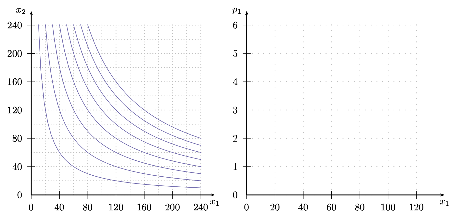
Good 1 - Good 2 Space
Two "Goods" : Good 1 and Good 2

1
Budget Constraints
2
Preferences
Definition Review:
Indifference Curves
Preferred/Dispreferred Sets
Marginal Rate of Substitution
3
Utility Functions
4
Indifference curve is
steeper than the budget line
Indifference curve is
flatter than the budget line
Moving to the right
along the budget line
would increase utility
Moving to the left
along the budget line
would increase utility
More willing to give up good 2
than the market requires
Less willing to give up good 2
than the market requires

The “Gravitational Pull" Towards Optimality
POINT A
POINT B
5
IF...
THEN...
The consumer's utility function is "well behaved" -- smooth, strictly convex, and strictly monotonic
The indifference curves do not cross the axes
The budget line is a simple straight line
The optimal consumption bundle will be characterized by two equations:
More generally: the optimal bundle may be found using the Lagrange method
Optimal Choice
6
Optimal Choice
Otherwise, the optimal bundle may lie at a corner,
a kink in the indifference curve, or a kink in the budget line.
No matter what, you can use the "gravitational pull" argument!
- Write an equation for the tangency condition.
- Write an equation for the budget line.
- Solve for \(x_1^*\) or \(x_2^*\).
- Plug value from (3) into either equation (1) or (2).

Solving for Optimality when Calculus Works
7
(Gross) demand functions are mathematical expressions
of endogenous choices as a function of exogenous variables (prices, income).
(Gross) Demand Functions
8
For a Cobb-Douglas utility function of the form
Special Case: The “Cobb-Douglas Rule"
The demand functions will be
That is, the consumer will spend fraction a/(a+b) of their income on good 1, and fraction b/(a+b) of their income on good 2.
This shortcut is very much worth memorizing! We'll use it a lot in the next few weeks in place of going through the whole optimization process.
9
Demand and Offer Curves
10
To Do Before Next Class
Be sure you're signed up for a section.
Do the reading and the quiz -- due at 11:15am on Thursday!
Read the syllabus carefully.
Look over the summary notes for this class.
11