Intertemporal Choice
Christopher Makler
Stanford University Department of Economics
Econ 51: Lecture 3
Today's Agenda
Part 1: Baseline Case
Part 2: Extensions and Applications
Modeling present-future tradeoffs
The intertemporal budget constraint
Preferences over time
Optimal saving and borrowing
Different interest rates for borrowing and saving
Credit constraints
Real and nominal interest rates
Beyond two time periods
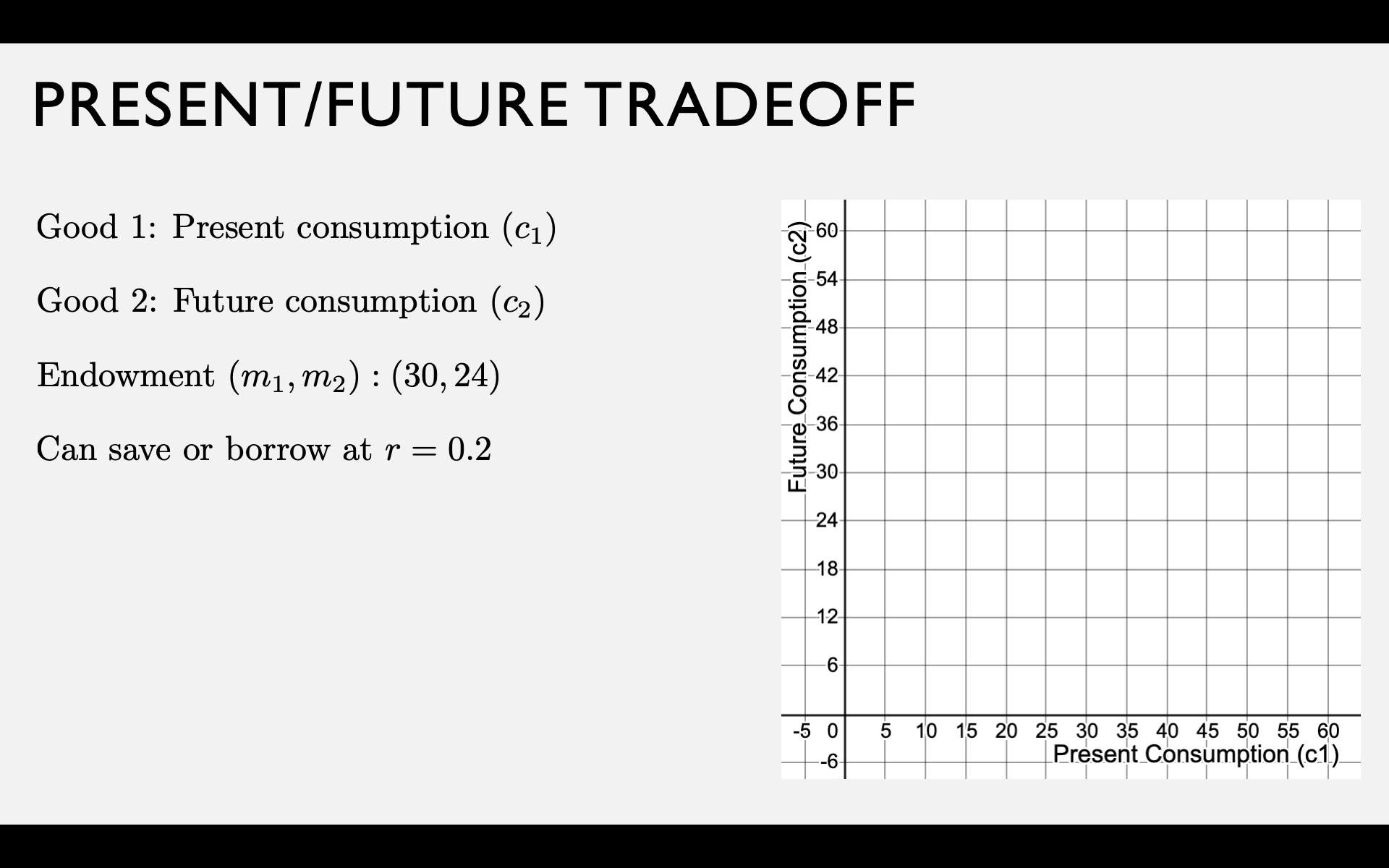
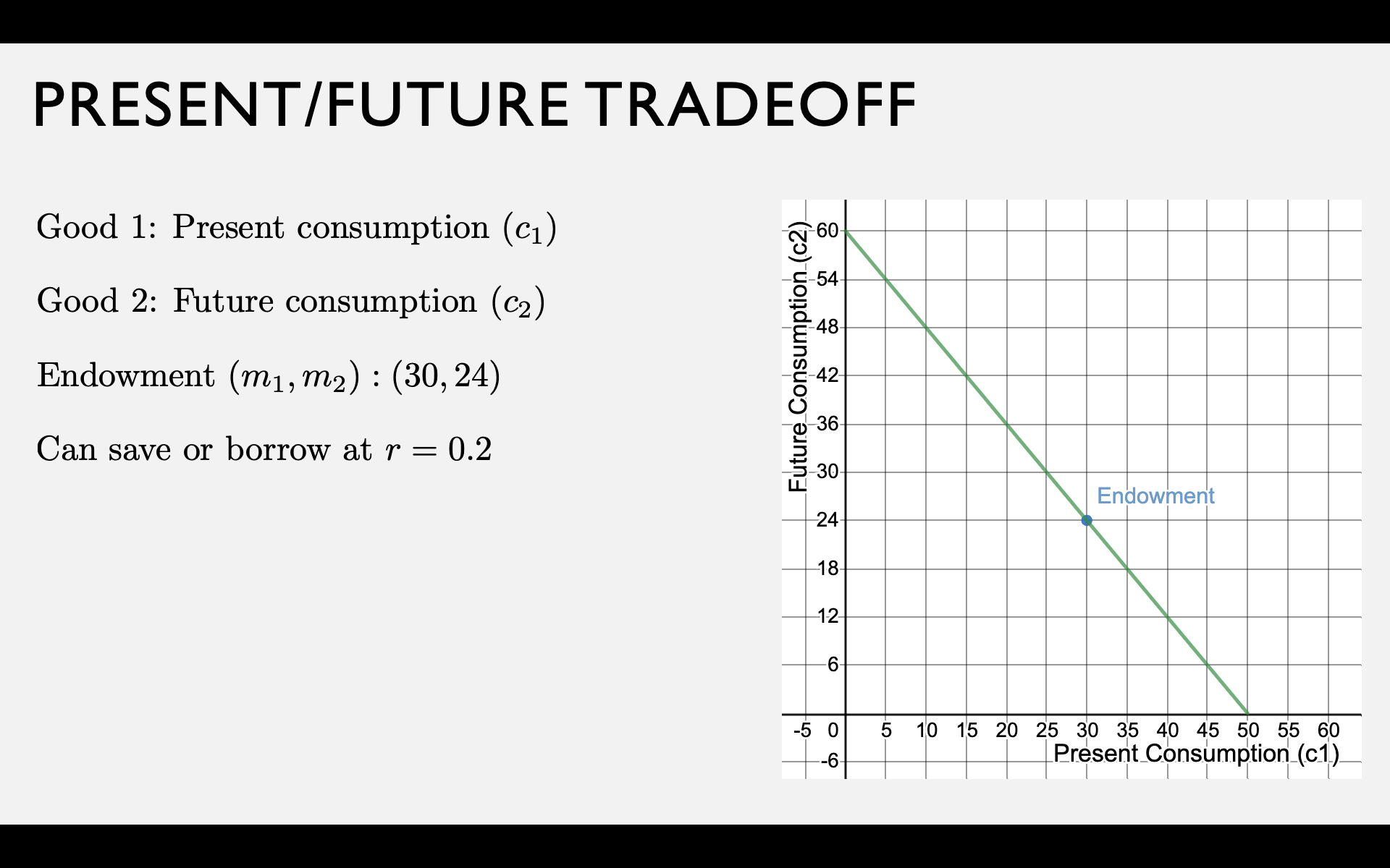
Saving and borrowing is a huge part of the U.S. economy.
Endowment of time and money.
Today: Present vs. Future Consumption
Endowment of money in different time periods (an "income stream")
Last time: Leisure vs. Consumption
Working = trading time for money
Saving = trading present consumption for future consumption
Borrowing = trading future consumption for present consumption
For Each Context:
Determine the budget line
Analyze preferences
Solve for optimal choice
Comparative statics: analyze net supply and demand
Do you have to spend all the money you earn in the period when you earn it?
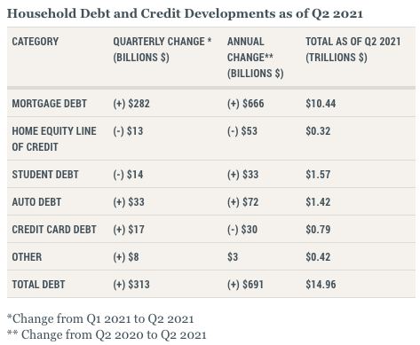
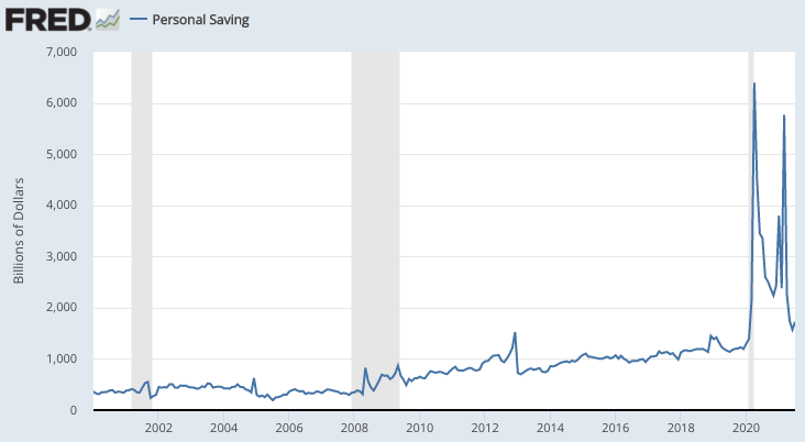
Present-Future Tradeoff
Your endowment is an income stream of \(m_1\) dollars now and \(m_2\) dollars in the future.
What happens if you don't consume all \(m_1\) of your present income?
Two "goods" are present consumption \(c_1\) and future consumption \(c_2\).
Let \(s = m_1 - c_1\) be the amount you save.
Saving and Borrowing with Interest
If you save at interest rate \(r\),
for each dollar you save today,
you get \(1 + r\) dollars in the future.
You can either save some of your current income, or borrow against your future income.
If you borrow at interest rate \(r\),
for each dollar you borrow today,
you have to repay \(1 + r\) dollars in the future.
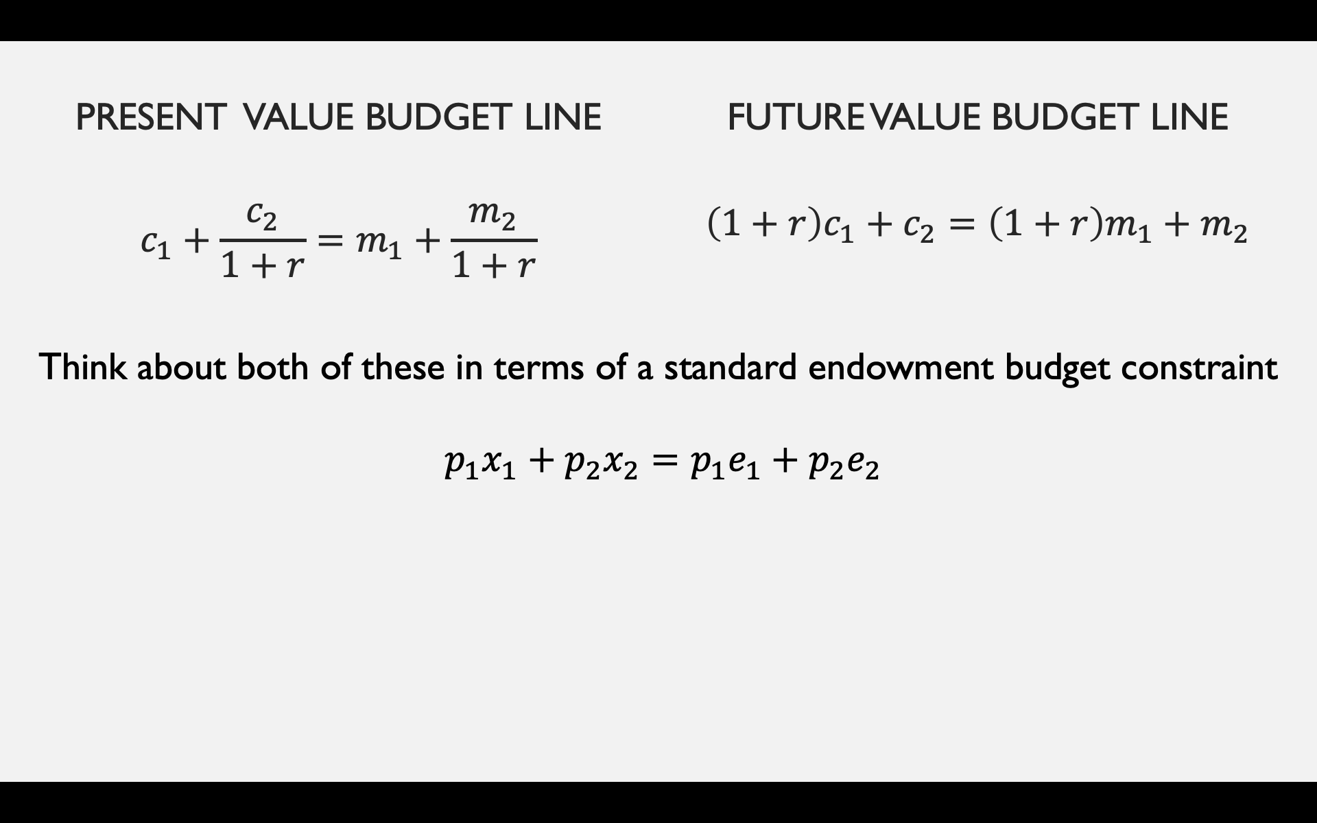
"Future Value"
"Present Value"
pollev.com/chrismakler

Preferences over Time
Examples:
When to borrow and save?
Save if MRS at endowment < \(1 + r\)
Borrow if MRS at endowment > \(1 + r\)
(high interest rates or low MRS)
(low interest rates or high MRS)
If we assume \(v(c)\) exhibits diminishing marginal utility:
MRS is higher if you have less money today (\(m_1\) is low)
and/or more money tomorrow (\(m_2\) is high)
MRS is lower if you are more patient (\(\beta\) is high)
Borrow or Save?
pollev.com/chrismakler
Optimal Bundle
Tangency condition:
Budget line:
pollev.com/chrismakler
Supply of Savings and
Demand for Borrowing
In general, net demand is \(x_1^* - e_1\)
In this context, net demand is the demand for borrowing.
If it's negative, then it's the supply of saving.
Different Buying and Selling Prices
BUY MORE GOOD 1
BUY LESS GOOD 1
Sell good 1 and buy good 2 if your MRS at the endowment is less than the price ratio to sell good 1 / buy more good 2.
Either way, it all comes down to the relationship between your MRS at the endowment and the relevant price ratios.
Buy good 1 and sell good 2 if your MRS at the endowment is greater than the price ratio to buy more good 1 / sell good 2
Different Interest Rates

When a Budget Line Ends...
Inflation and Real Interest Rates
"Present Value" for two periods
"Present Value" for three periods
Why stop at two periods?
Net Present Value
Application: Social Cost of Carbon
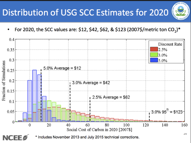
Obama Admin: $45
Uses a 3% discount rate; includes global costs
Trump Admin: less than $6
Uses a 7% discount rate; only includes American costs
PV of $1 Trillion in 2100:
$86B for Obama, $4B for Trump