Machine Learning Introduction
Introduction
1
Introduction
2
- Fundamentals
-
Introduction Supervised Learning
- Neural Nets with AND
- MNIST
-
Introduction Unsupervised Learning
- K-Means Clustering
-
Introduction Reinforcement Learning
- Q-Learning
- Summary
Structure
Fundamentals
3
Fundamentals
- What is ML?
- Why do we need it?
- What are the use cases?
- Do I need a Ph.D to understand all of this?
Supervised Learning
4
Supervised Learning
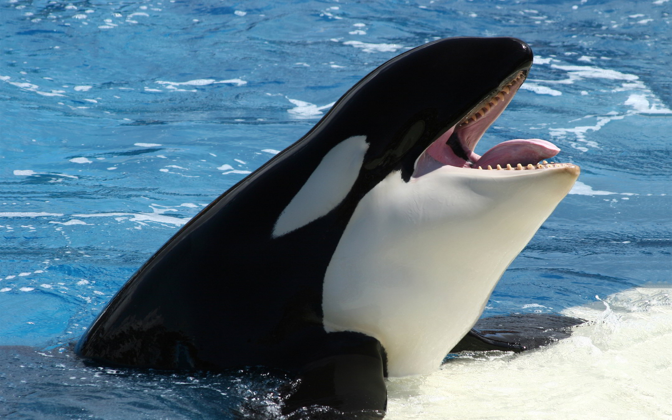
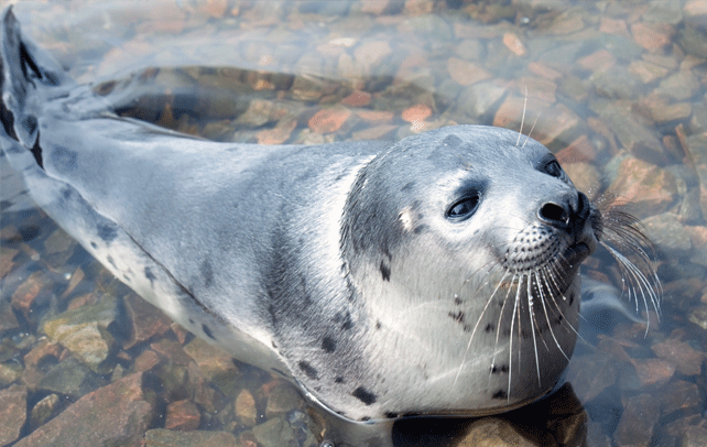
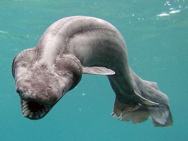
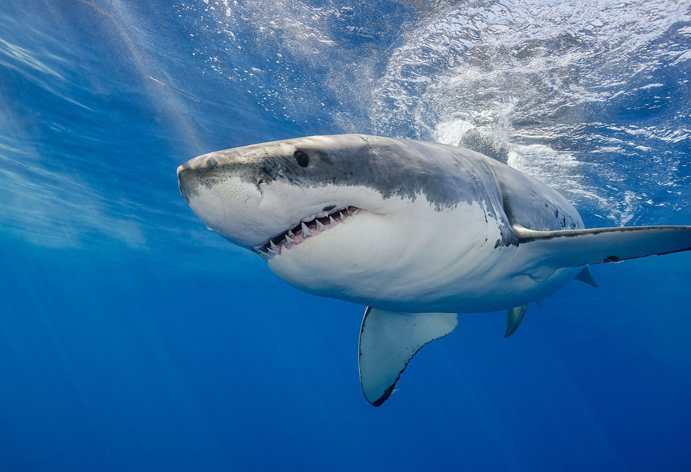
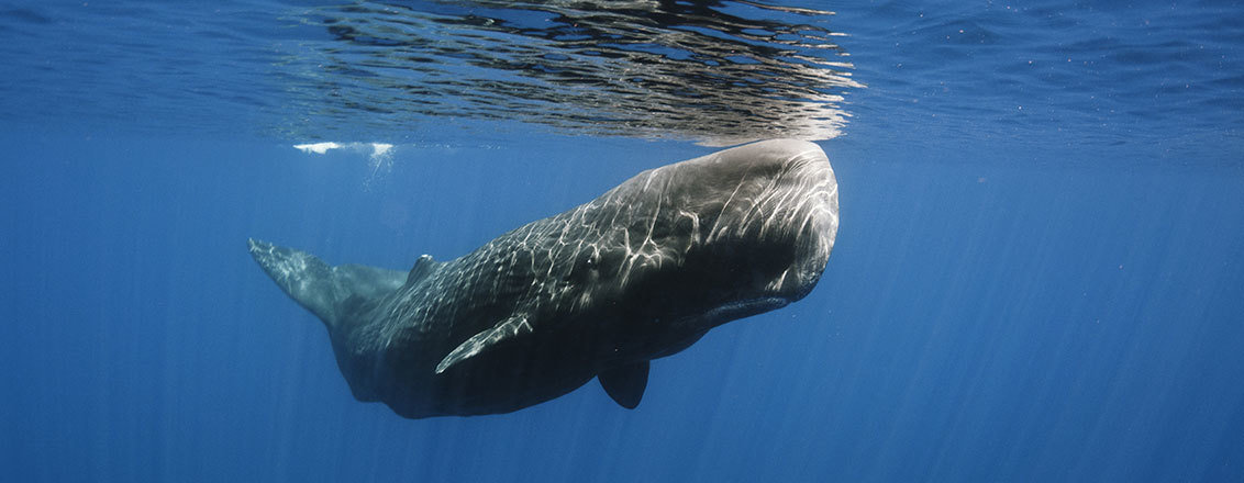
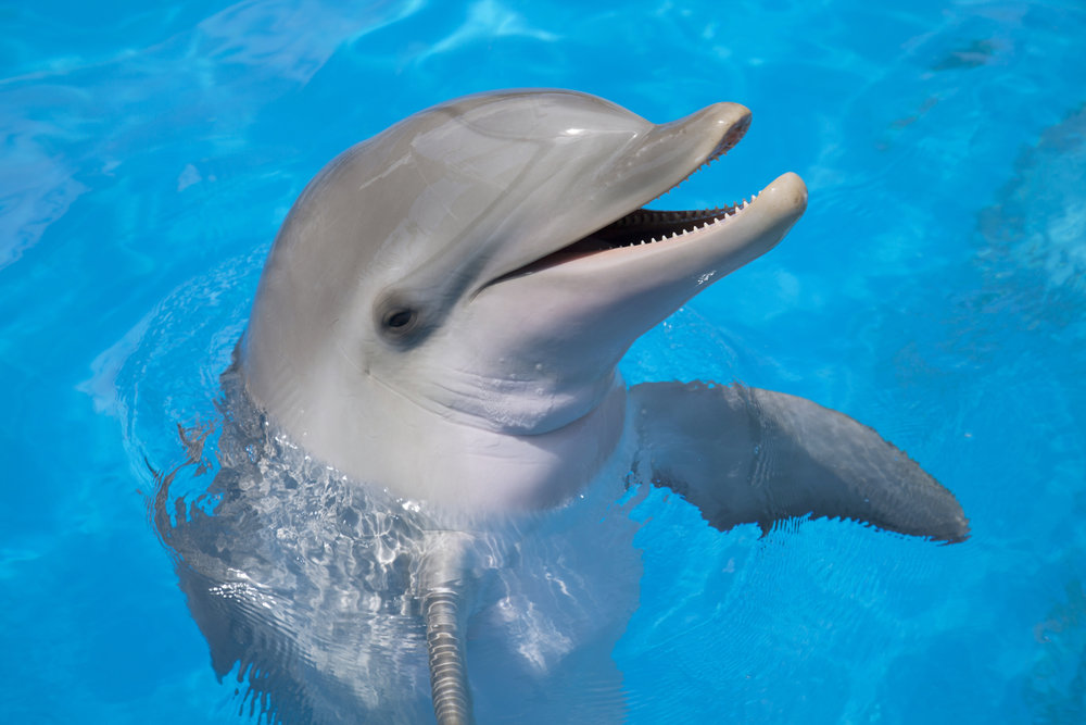
Mammal
Not a mammal
Mammal?
Supervised Learning
5
Logical AND - Problem
x1
x2
0
1
0
1
| x1 | x2 | ∧ |
|---|---|---|
| 0 | 0 | 0 |
| 0 | 1 | 0 |
| 1 | 0 | 0 |
| 1 | 1 | 1 |
∧ = 0
∧ = 1
0
0
0
1
Supervised Learning
6
Logical AND - Problem
x1
x2
0
1
0
1
h < 0
h >= 0
How to learn such a function?
Supervised Learning
7
Perceptron
Supervised Learning
8
Perceptron for AND
< 0: 0 (false)
>= 0: 1 (true)
Supervised Learning
9
Perceptron for AND
0 = false
1 = true
Input:
Randomly choosen weights:
x1
x2
0
1
0
1
Supervised Learning
10
Cost Function
| x_1 | x_2 | y | ^y | C |
|---|---|---|---|---|
| 0 | 0 | 0 | 0 | 0 |
| 0 | 1 | 0 | 1 | -1 |
| 1 | 0 | 0 | 1 | -1 |
| 1 | 1 | 1 | 1 | 0 |
x1
x2
0
1
0
1
-1
-1
Supervised Learning
11
Backpropagation
-1
0
0
1
Update rule:
Supervised Learning
12
Backpropagation
Misclassified:
Update rule:
Learning rate:
Weights:
Supervised Learning
13
Test
x1
x2
0
1
0
1
Supervised Learning
14
Summary
x1
x2
0
1
0
- Get labeled data (AND - Table)
- Run the data and calculate the error
- Use partial deriviative of cost function to create a learning rule
- For every mislabled sample, apply learning rule
- Hope that it's linear separable
XOR
1
Supervised Learning
15
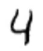
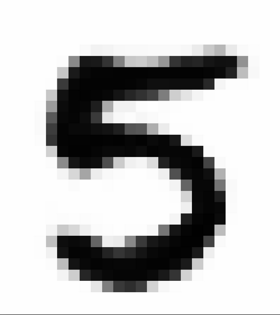
Example - MNIST
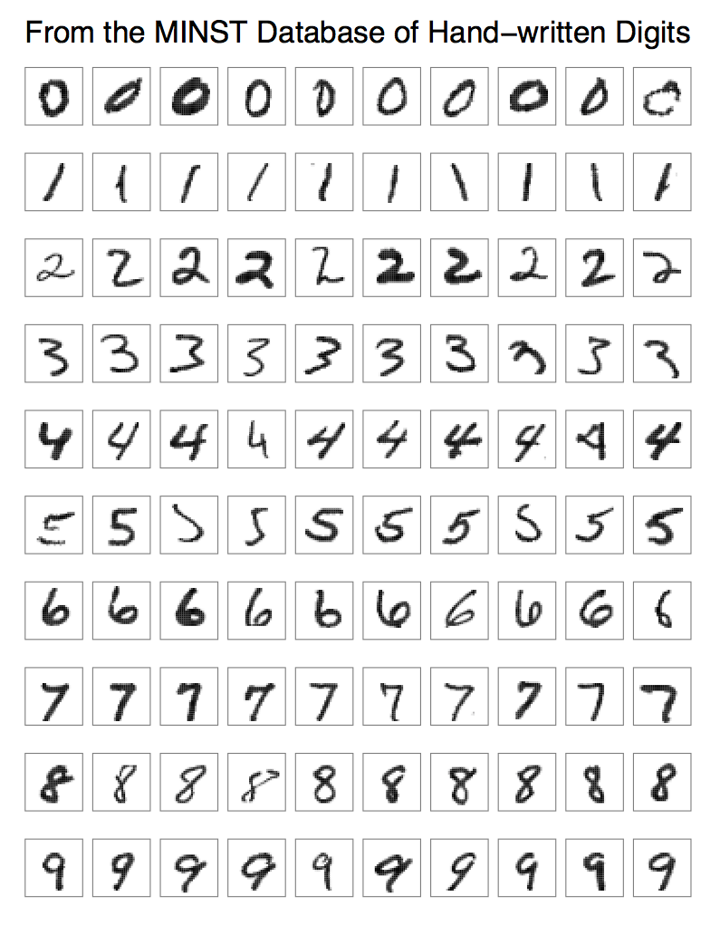
?
13% #0
0% #1
5% #2
1% #3
67% #4
2% #5
2% #6
3% #7
3% #8
4% #9
Supervised Learning
16
Example - MNIST
?
13% #0
0% #1
5% #2
1% #3
67% #4
2% #5
2% #6
3% #7
3% #8
4% #9
Supervised Learning
17
Multiple Perceptrons
b/w pixel data

13% #0
0% #1
5% #2
1% #3
67% #4
2% #5
2% #6
3% #7
3% #8
4% #9
Supervised Learning
18
Linear Separable
Index
b/w
Supervised Learning
19
Multiple Layers of Perceptrons
b/w pixel data
13% #0
0% #1
5% #2
1% #3
67% #4
2% #5
2% #6
3% #7
3% #8
4% #9
Supervised Learning
20
Additional Information
- Convolutional Networks
- Recurrent Networks
- LSTM Neurons
Supervised Learning
21
Neural Style Transfer
https://handong1587.github.io/deep_learning/2015/10/09/fun-with-deep-learning.html
Supervised Learning
22
Neural Photorealistic Style Transfer
https://github.com/luanfujun/deep-photo-styletransfer


Supervised Learning
23
Text to Speech
Normal text
Randomly generated text
Music
https://deepmind.com/blog/wavenet-generative-model-raw-audio/
Unsupervised Learning
24
Unsupervised Learning
Feature 1
Feature 2
Feature 1
Feature 2
Unknown structure
Known structure
Unsupervised Learning
25
K - Means Clustering
Feature 1
Feature 2
Unsupervised Learning
26
K - Means Clustering
Feature 1
Feature 2
Unsupervised Learning
27
K - Means Clustering
Feature 1
Feature 2
Unsupervised Learning
28
K - Means Clustering
Feature 1
Feature 2
Unsupervised Learning
29
K - Means Clustering - Caveats
Feature 1
Feature 2
- Amount of clusters
Unsupervised Learning
30
K - Means Clustering - Caveats
Feature 1
Feature 2
- Amount of clusters
- Similarity measure
Unsupervised Learning
31
K - Means Clustering - Caveats
Feature 1
Feature 2
- Amount of clusters
- Similarity measure
- No convergence
Unsupervised Learning
32
Additional Information
- Principal Component Analysis
- Support Vector Machines
- Autoencoder
Unsupervised Learning
33
K-Means Clustering of 40K samples of homework
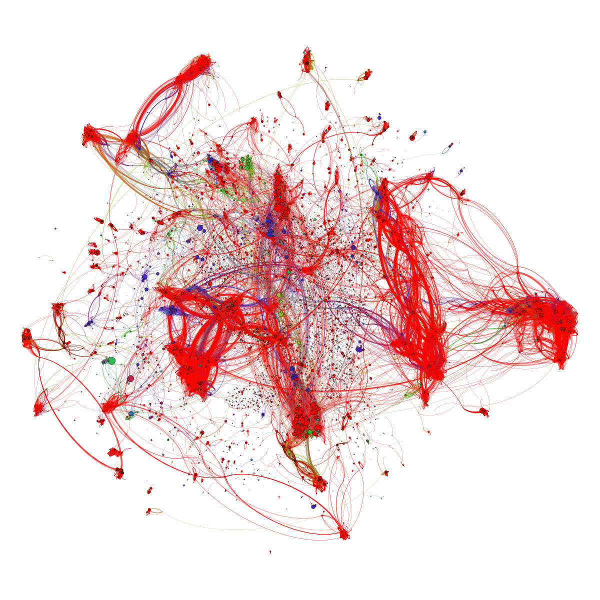
http://practicalquant.blogspot.de/2013/10/semi-automatic-method-for-grading-a-million-homework-assignments.html
Reinforcement Learning
34
Reinforcement Learning
Environment
Agent
Action
State
Reward
Reinforcement Learning
35
Formalizing RL
Environment
Agent
Action
State
Reward
Reinforcement Learning
36
Formalizing RL
Environment
Agent
Action
State
Reward
Reinforcement Learning
37
Reward
Environment
Agent
Action
State
Reward
Reinforcement Learning
38
Timed Reward
Environment
Agent
Action
State
Reward
Reinforcement Learning
39
Discount Rate
Environment
Agent
Action
State
Reward
Reinforcement Learning
40
Discount Rate
Environment
Agent
Action
State
Reward
Reinforcement Learning
41
Short-Sighted Reward
Environment
Agent
Action
State
Reward
Reinforcement Learning
42
Balanced Rewards
Environment
Agent
Action
State
Reward
Reinforcement Learning
43
Q(uality) - Learning
Environment
Agent
Action
State
Reward
Represents the quality of an action in the current state, while continuing to play optimally from that point on
Reinforcement Learning
44
Q(uality) - Learning
Problem: How to construct such a Q function?
Reinforcement Learning
45
Bellmann Equation
Maximal reward is defined as immediate reward + maximum future reward for next state
Reinforcement Learning
46
Learning Q-Function
Reinforcement Learning
47
Learning Q-Function
Reinforcement Learning
48
Learning Q-Function with NNs
NN
Reinforcement Learning
49
Additional Information
Experience Replay
Exploration - Exploitation
Slides adapted from excellent tutorial
https://www.nervanasys.com/demystifying-deep-reinforcement-learning/
Reinforcement Learning
50
TORCS
https://yanpanlau.github.io/2016/10/11/Torcs-Keras.html
Reinforcement Learning
51
Buzzwords we learned today
Perceptron
Backpropagation
Neural Nets
Supervised Learning
MNIST Dataset
Linear Separable
Unsupervised Learning
Clustering
K-Means
Distance Measures
Convergence
RL Learning
Policy
Q-Learning
Discount Rate
TORCS
Reinforcement Learning
52
Imagesources
- Cetacea - http://www.toggo.de/media/slider-wal-3-14295-10110.jpg
- Orca - http://elelur.com/mammals/orca.html
- Pinniped - http://www.interestingfunfacts.com/amazing-facts-about-pinniped.html
- Deep Sea Frill Shark - http://images.nationalgeographic.com/wpf/media-live/photos/000/181/cache/deep-sea01-frill-shark_18161_600x450.jpg
- Shark - http://www.livescience.com/55001-shark-attacks-increasing.html
- Dolphin - http://weknownyourdreamz.com/dolphin.html