Bernardo Aceituno,
Carlos Mastalli,
Hongkai Dai,
Michele Focchi,
Andreea Radulescu,
Darwin G. Caldwell,
Jose Cappelletto,
Juan C. Grieco,
G. Fernandez-Lopez,
Claudio Semini
Centroidal Dynamic Model
- Non-coplanar stability through friction cone constraints
- The centroidal dynamics describes the system's evolution
- Integer variables model the contacts and gait transitions
- Approximate the robot's joint torque limits
We represent the time evolution of the system using a centroidal dynamics model [1]
where
- CoM position
- Angular Momentum
- Contact force of end-effector
- Position of end-effector
Centroidal Dynamic Model
[1] Orin et al., "Centroidal dynamics of a humanoid robot", 2013
We represent the time evolution of the system using a centroidal dynamics model
The non-linear term can be described as bilinear function [2], and it can be decomposed as:
Centroidal Dynamic Model
[2] Ponton et al., "A Convex Model of Momentum Dynamics for Multi-Contact MotionGeneration", 2013
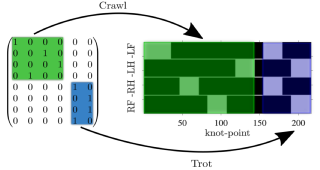
A gait matrix [3] describes when i contact swings in determined time-slot j :
Since each contact location in the plan is reached once, we enforce:
Contact and Gait Sequence
- Number of contacts
- Number of time-slots
[3] Aceituno-Cabezas et al., “A Mixed-Integer Convex Optimization Framework for Robust Multilegged
Robot Locomotion Planning over Challenging Terrain”, 2017
Once is assigned the contact to swing, we optimize the contact locations, represented as 4D vectors:
and then, we assign this contact to one of the by using a binary matrix :
Contact and Gait Sequence
where the (implies) operator is represented with big-M formulation.
[3] Aceituno-Cabezas et al., “A Mixed-Integer Convex Optimization Framework for Robust Multilegged
Robot Locomotion Planning over Challenging Terrain”, 2017
We approximate the kinematic limits as a bounding box with respect to the CoM. Algebraically:
where
- CoM position at i transition
- Diagonal of the bounding box
- Distance from the trunk of leg
Contact and Gait Sequence
and the trigonometric functions are decomposed in piecewise linear
functions [4].
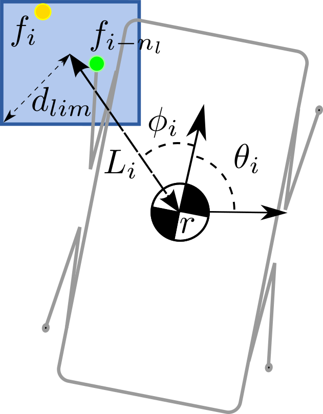
[4] Deits and Tedrake, “Footstep Planning on Uneven Terrain with Mixed-Integer Convex Optimization”, 2014
We define as swing reference trajectory, connected to adjacent
contacts, where:
- j indicates the time-slot, and
- all the knots per time-slot
Contact and Gait Sequence
This constraint enforces that the leg reaches the contact position at
the end of the j slot

with:
The leg number for the i contact
For stance condition, we constraint the leg to remain stationary as:
- are the contact indexes assigned to the l leg
Contact and Gait Sequence
where
If a swing is activated on l leg, there is no contact force:
Contact and Gait Sequence
where is the set of knots in the j slot used for the swing.
This can be see as complementary constraint [5,6]
[5] Stewart and Trinkle, “An implicit time-stepping scheme for rigid body dynamics with Coulomb friction”, 2000
[6] Mastalli et al., “Hierarchical Planning of Dynamic Movements without Scheduled Contact Sequences”, 2016
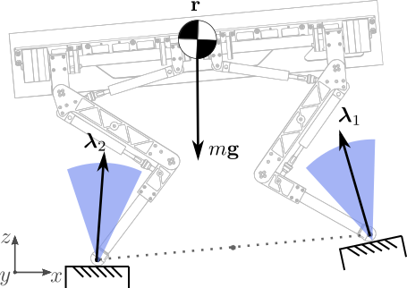
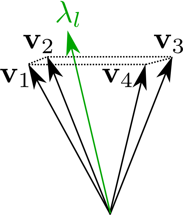
We add robustness to this condition because we maximize a lower bound of the distance of the force vector to each cone edge as:
Contact and Gait Sequence
where are positive multipliers on each cone edge
We can ensure stability on arbitrary terrain with non-coplanar contacts by incorporating linearized friction cone constraints:
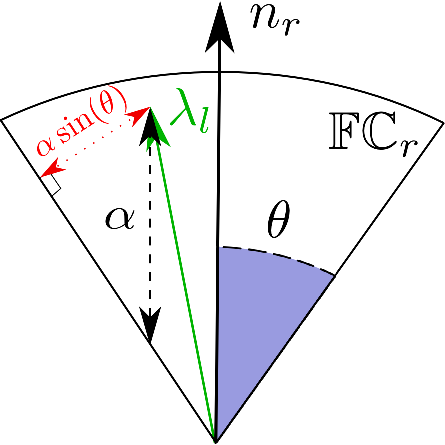
Contact and Gait Sequence
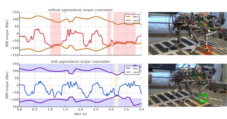
We approximate joint torque limits by using a nominal value of the Jacobian :
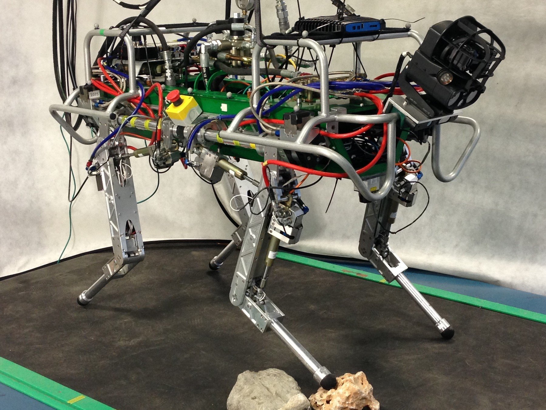
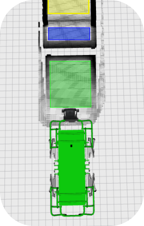
HyQ Crossing Terrain with Various Slopes