Decoding Your Data

Decoding Skewness : Understanding Data Distribution


Learning Outcome
6
Compute skewness using Python
5
Interpret positive and negative skew
4
Define skewness mathematically and conceptually
3
Understand symmetry in distributions
2
Explain the bell-curve concept
1
Define a statistical distribution
Statistical concepts to Recall
Mean, Median, Mode
measure of central tendency
Standard Deviation
measures the spread of data
Variance
Average of squared deviations from the mean
Concept of outliers
Understanding and identifying data points that differ significantly from the rest


Imagine a teacher drawing students' marks on a graph.
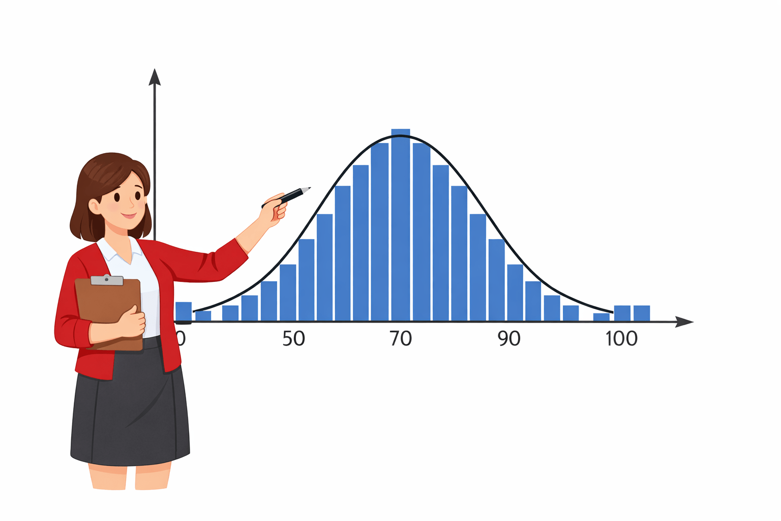
In one class:
- Most students score around 70.
- Very few score low.
- Very few score high.
The graph looks balanced.
In another class:
- Most students score high.
-
But a few score extremely low.
The graph leans to one side.
Even if the average marks look similar in both classes, the shape of the graph is different.
And that shape difference is important.
When that shape leans to one side, we call it Skewness.
The average might look similar.
The way data spreads on a graph is called its shape.
To understand skewness, we must first understand:
-
What is a distribution?
-
What does symmetry mean?
-
What is the normal (bell-shaped) distribution?
Only then can we understand how distributions become tilted.

What is a Distribution?
A distribution describes how data values are arranged across possible outcomes.
Instead of looking at individual numbers, we look at:
- How often values appear (frequency)
- Where most values are grouped (cluster)
- How spread out the values are (spread)
Example:
Marks: 40, 55, 60, 70, 70, 75, 80, 90
If we draw these in a histogram (bar graph), we don’t just see numbers — we see a pattern.
📍 Many students scored around 70–80 → values are clustered in the middle
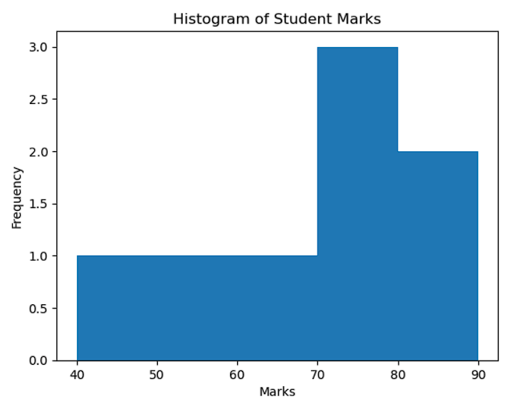
This overall pattern is called the distribution.
📍 Most marks are between 60 and 80
📍 Very few students scored very low (40) or very high (90)
From this, we can understand:

Distribution Helps Us Answer:
- Is the data centered?
- Is it symmetric?
- Are extreme values common?
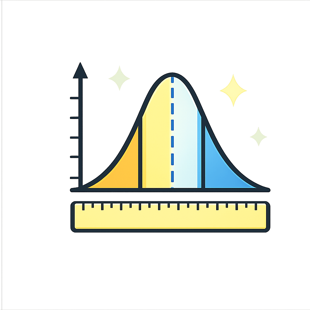
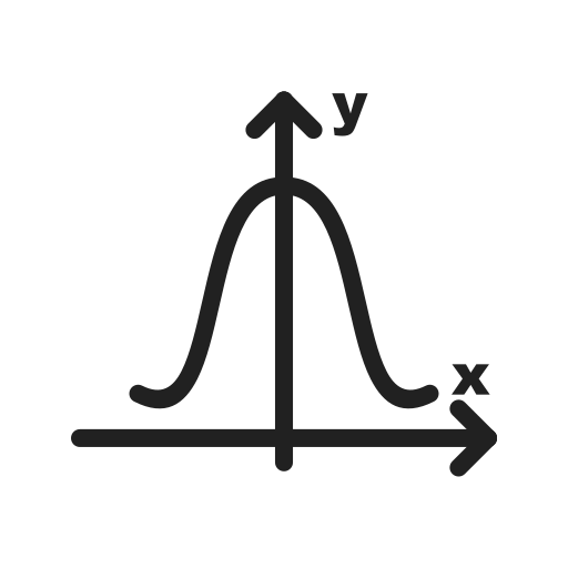
The Bell Curve (Normal Distribution as Baseline)
The Normal Distribution is the most common and important distribution in statistics.
It is often called the Bell Curve because of its shape.
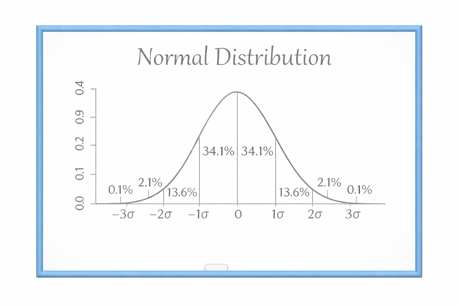
Why is it called a Bell Curve?
It looks like a bell:
-
High in the middle
-
Low on both sides
-
Perfectly balanced
Main Characteristics

Bell-Shaped
The graph rises in the middle and falls smoothly on both sides.

Perfectly Symmetric
Left side = Right side
If you fold it in half, both sides match.

Mean = Median = Mode
All three are exactly at the center.

Defined by Only Two Things
-
Mean (μ)
-
Standard deviation (σ)

Conceptually :
- Most values lie near the mean
-
Probability decreases smoothly as we move away
-
Tails approach zero but never touch it
Mathematically, its probability density function is:
f(x) = (1 / (σ√2π)) e^(-(x-μ)² / (2σ²))

Normal distribution acts as the benchmark for symmetry.
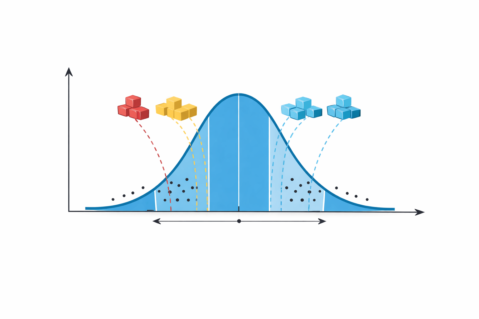
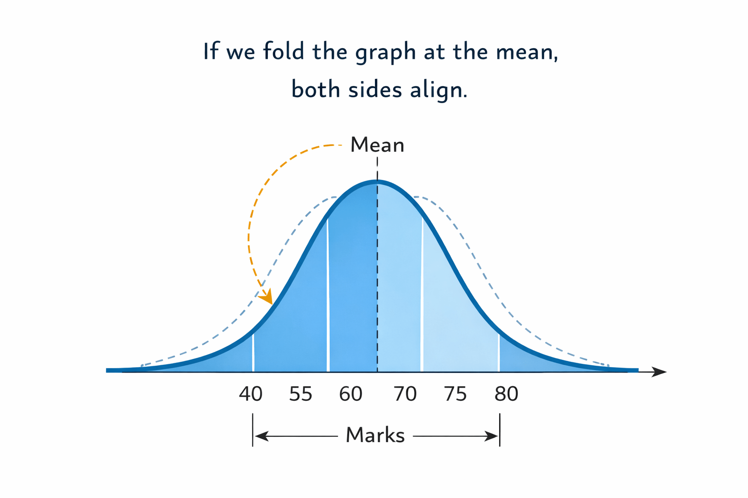
Symmetry in Distribution
A distribution is symmetric if:
Left half mirrors the right half around the mean.
In symmetric distributions:
Mean = Median = Mode
If we fold the graph at the mean, both sides align.
Skewness measures departure from this symmetry.
What is Skewness?
Skewness tells us whether data is tilted to one side.
It measures:
- Direction of tilt
-
Degree of asymmetry
- If data is perfectly balanced → skewness = 0
- If data leans to one side → skewness ≠ 0
Mathematical Formula (Population Skewness):
Skewness = E[(X − μ)³] / σ³

Why cube (³)?
- Squaring removes direction
-
Cubing preserves sign
If deviations on one side dominate,
the cube amplifies that direction.
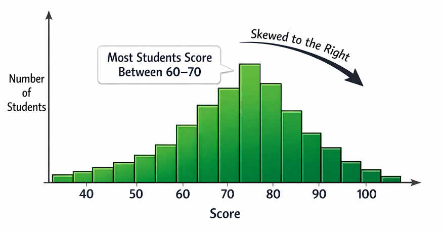
Positive Skewness (Right-Skewed Distribution)
Right tail is longer.
Extreme values exist on the higher side.
Student Example
Most students score between 60–70.
Statistical Property
Mean > Median > Mode
Reason:
- Large high values pull mean upward.
- Median moves less.
- Mode stays near peak.
Interpretation
Positive skew suggests:
- Risk of extreme high values
- Long right tail
import numpy as np
from scipy.stats import skew

data = np.array([60, 65, 70, 68, 67, 100])

print("Skewness:", skew(data))

# If result > 0 → Positive skew.
Python Example
OUTPUT
Skewness:

1.553857733074746

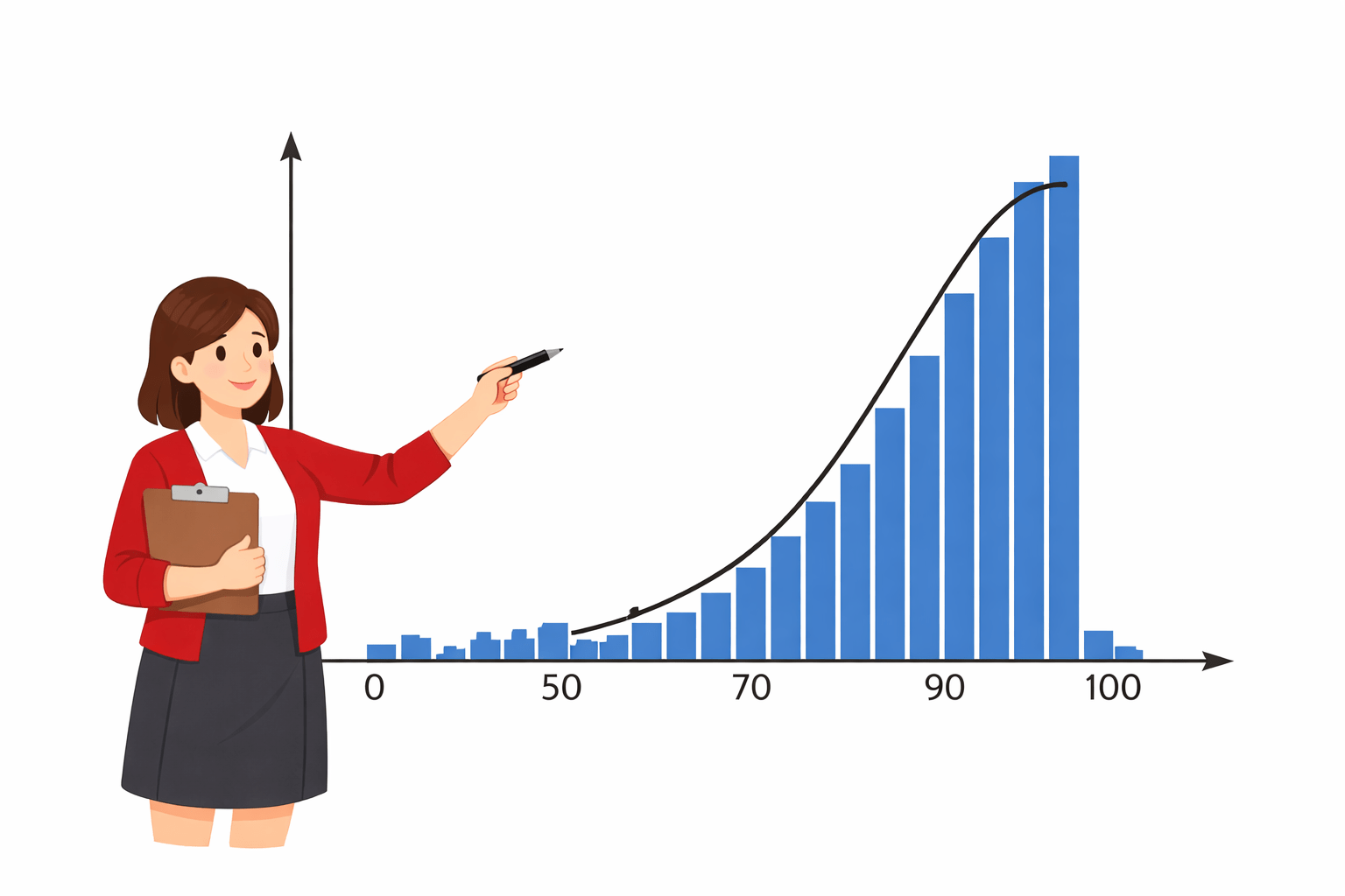
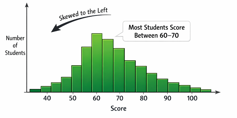
Negative Skewness (Left-Skewed Distribution)
Left tail is longer.
Extreme low values dominate.
Student Example
Most students score between 70–80.
Statistical Property
Mean < Median < Mode
Reason:
-
Low values pull mean downward.
Python Example
import numpy as np
from scipy.stats import skew

data = np.array([70, 75, 80, 78, 76, 20])

print("Skewness:", skew(data))

# If result < 0 → Negative skew.
OUTPUT
Skewness:
-1.7052408586537422
Interpreting Skewness Values
Skewness ≈ 0 → Symmetric
-
Data is balanced.
-
Left side ≈ Right side.
-
Mean ≈ Median ≈ Mode.
No tilt.
Mild asymmetry.
0.5 < |skew| < 1 → Moderately Skewed
-
Data is slightly tilted.
-
One side is longer than the other.
-
Not extreme, but noticeable.
|skew| > 1 → Highly Skewed
-
Strong tilt.
-
One tail is much longer.
-
Extreme values are pulling the data heavily to one side.
Strong asymmetry.
What is Kurtosis?
Skewness measures tilt.
Kurtosis measures tail heaviness and extremity.
It tells us:
- How frequently extreme deviations occur.
Mathematical Formula :
Kurtosis = E[(X − μ)⁴] / σ⁴

Why fourth power?
-
Fourth power exaggerates extreme values strongly.
-
Large deviations increase kurtosis dramatically.
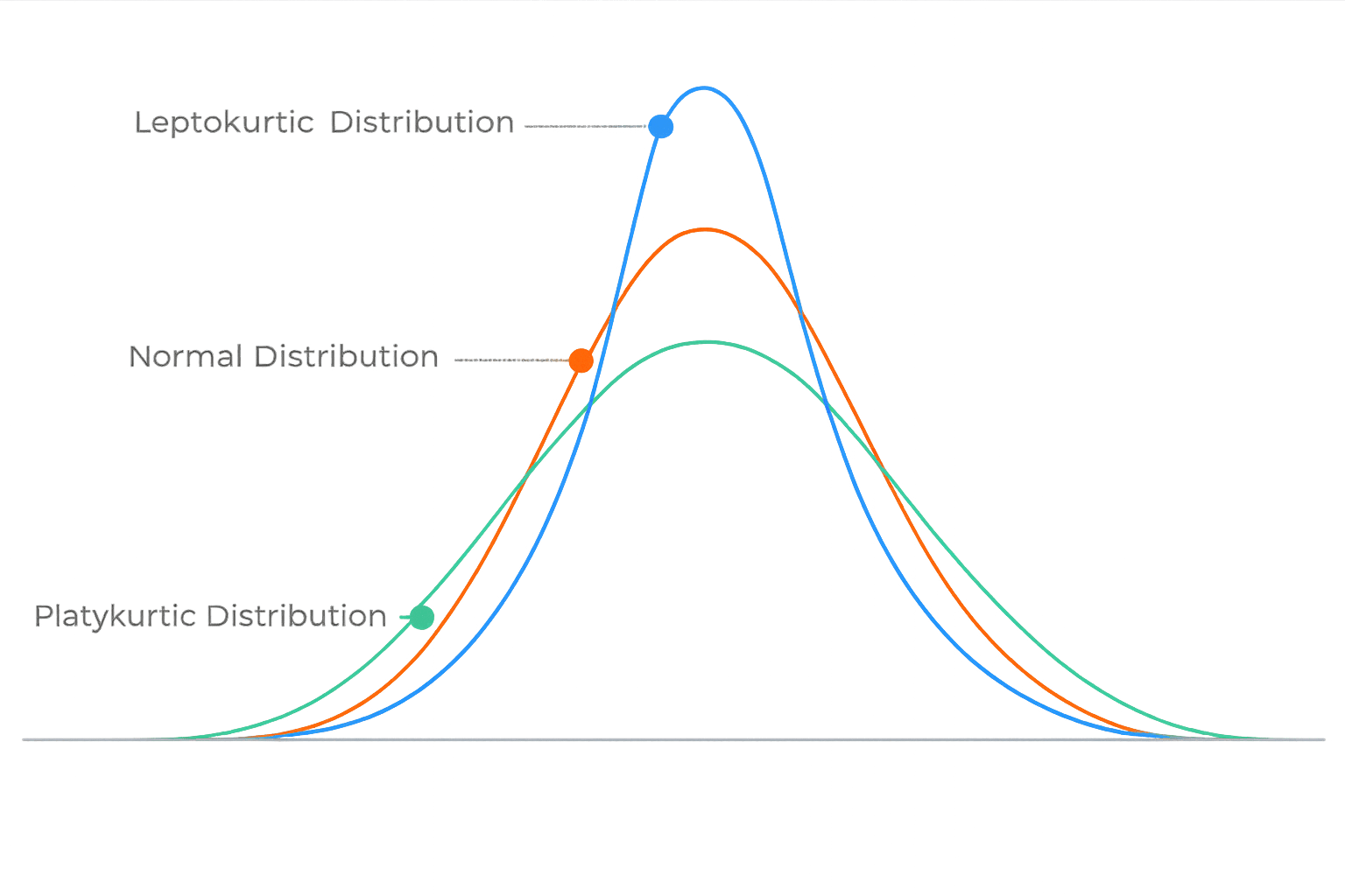
Types of Kurtosis
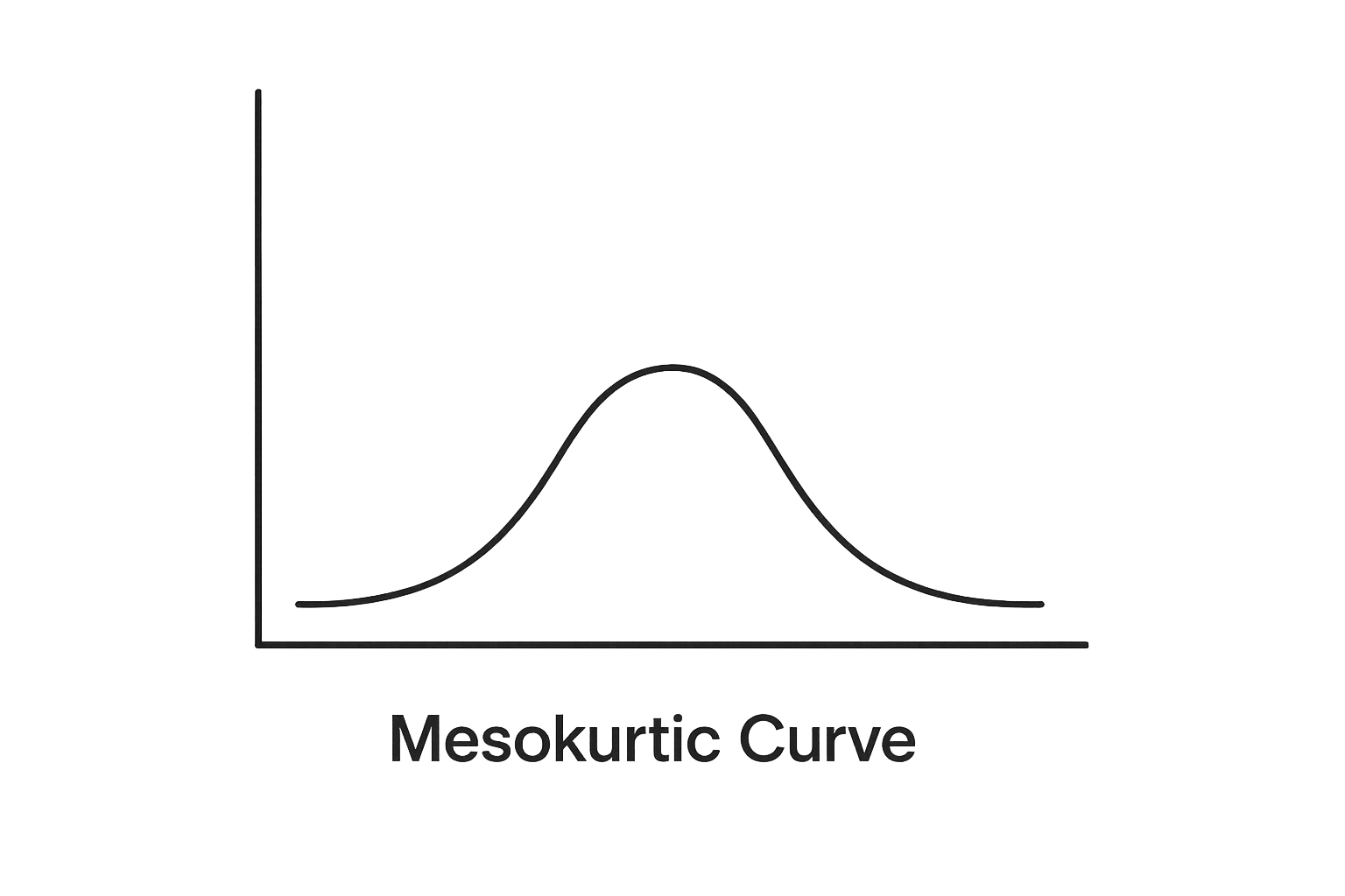
(A) Mesokurtic
Mesokurtic means the distribution has normal (medium) tails.
It is the same kurtosis as a normal distribution.
Key Points
Normal distribution
Moderate tails (not too heavy, not too light)
Extreme values are neither too many nor too few
Excess kurtosis = 0


(B) Leptokurtic (High Kurtosis)
Leptokurtic means the distribution has heavy tails.
Key Characteristics :
Heavy tails
More extreme values
Higher peak
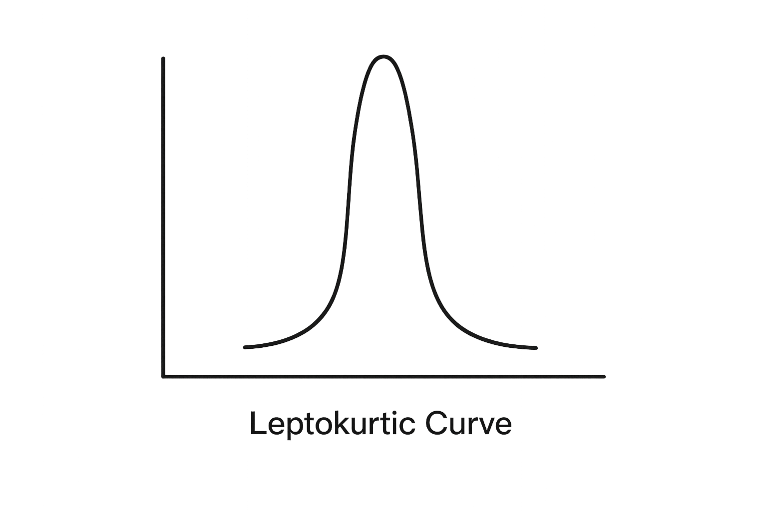
Interpretation:
- Higher probability of extreme outcomes.
- Common in financial returns.
(C) Platykurtic (Low Kurtosis)
Platykurtic means the distribution has thin tails.
Key Characteristics :
Thin tails
Fewer extreme values
Flatter peak
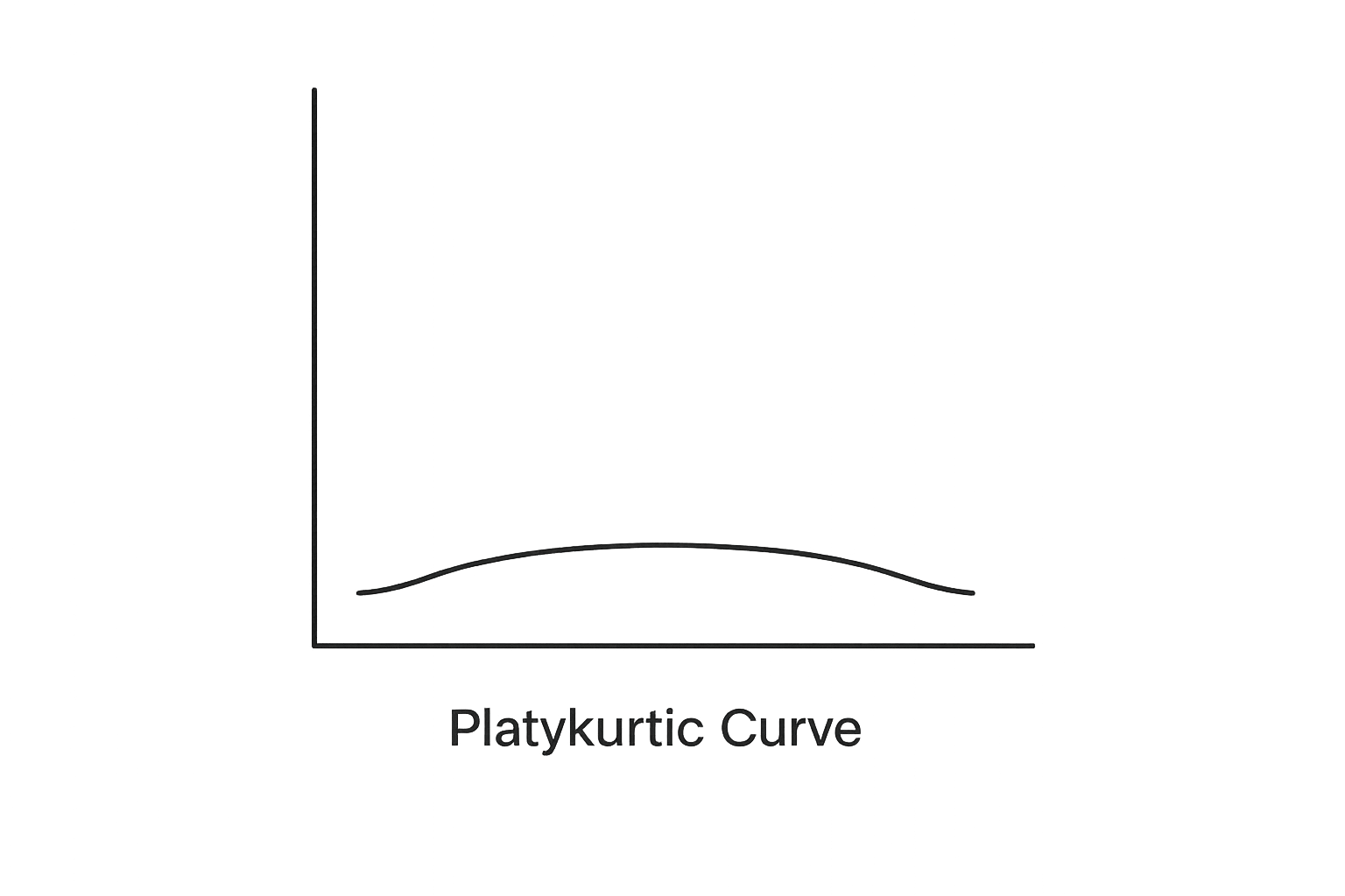
Interpretation:
- Data is more evenly spread.
Excess Kurtosis
Most software reports:
Excess Kurtosis = Kurtosis − 3

Why subtract 3?
Because normal distribution has kurtosis = 3.
So:
- Excess Kurtosis > 0 → Heavy tails
- Excess Kurtosis < 0 → Light tails
Python Example
import numpy as np
from scipy.stats import kurtosis

data = np.array([60, 65, 70, 68, 67, 100])

print("Excess Kurtosis:", kurtosis(data))
OUTPUT
Excess Kurtosis: 0.8286025196163282
Why Shape Matters in Analysis?
Many statistical methods assume normal distribution.
Shape affects:
Reliability of mean
Risk estimation
Confidence intervals
Hypothesis testing
Machine learning models
1
2
3
4
5

If data is skewed or heavy-tailed:
Mean may mislead
Standard deviation may underrepresent risk
Transformations may be required


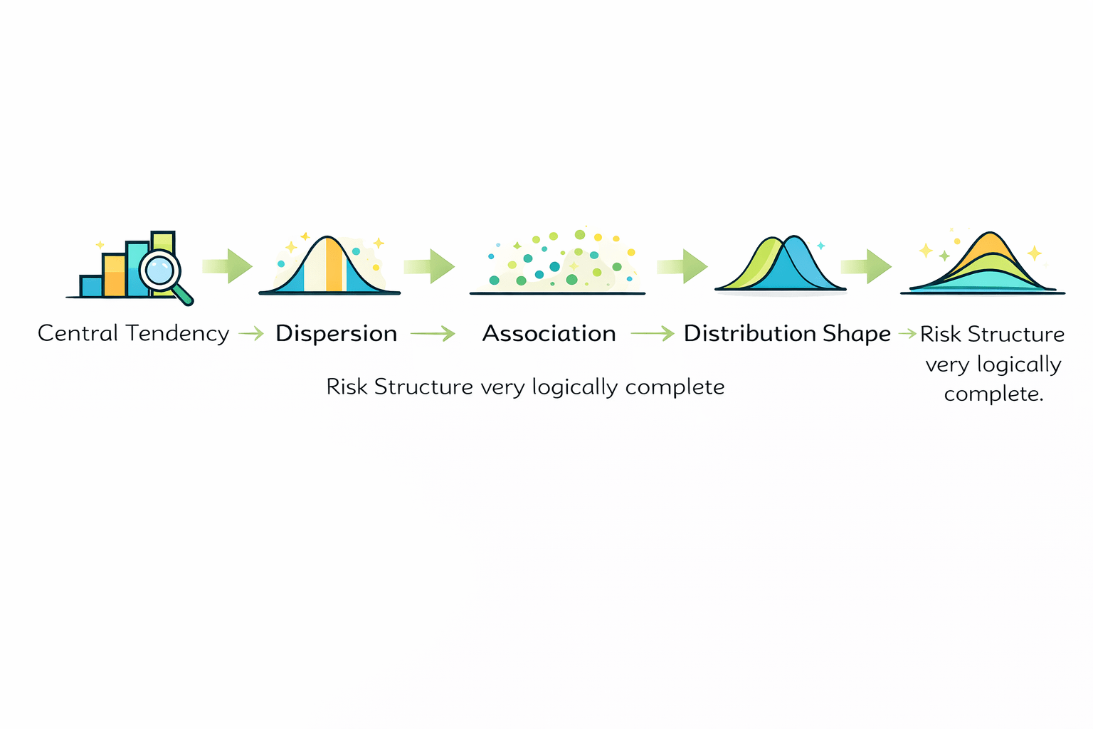
Why This Integration Matters
When analyzing real-world data, a structured approach improves accuracy:

Find the center → Understand typical behavior

Measure spread → Understand stability

Examine relationships → Understand interactions

Check skewness → Validate symmetry assumption


Check kurtosis → Evaluate risk of extremes
Only after all five steps can we confidently:
Build predictive models
Perform hypothesis testing
Make financial or business decisions
Train machine learning models

Ignoring any of these layers can lead to:
Biased conclusions
Underestimated risk
Incorrect predictions

Statistics is not just about calculation.
It is about understanding structure before drawing conclusions.
This integration section now makes the progression:
Summary
5
Distribution shape impacts statistical modeling
4
Kurtosis measures tail heaviness
3
Skewness measures asymmetry
2
Normal distribution is symmetric bell curve
1
Distribution describes arrangement of values
Quiz
Positive skew implies:
A. Mean < Median
B. Mean > Median
C. No tail
D. Flat distribution

Quiz-Answer
Positive skew implies:
A. Mean < Median
B. Mean > Median
C. No tail
D. Flat distribution