BIOSC 1540: L10A (Atomistic insight)
This is a live streamed presentation. You will automatically follow the presenter and see the slide they're currently on.
This is a live streamed presentation. You will automatically follow the presenter and see the slide they're currently on.
Computational Biology
(BIOSC 1540)
Mar 18, 2025
Lecture 10A
Atomistic insight
Foundations
Assignments
Quizzes
Final exam
When you are finished, please hold on to your quiz and feel free to doodle or write anything on the last page
Macrostates
Number of Particles: Biological systems contain billions of atoms interacting simultaneously
Thermal Motion: Atoms and molecules are in constant motion due to thermal energy
Uncertainty and Variability: Exact positions and velocities of particles are inherently uncertain
Microscopic level: Individual atoms and molecules
Macroscopic level: Bulk properties from collective behavior
Atomistic systems are stochastic, measurable properties are computed as averages
Statistical mechanics uses statistical methods to relate microscopic properties to macroscopic observables
Changing any one of these values changes the macrostate
A macrostate is defined by macroscopic variables such as temperature, pressure, volume, and number of particles.
Example: Methanol and water
Composition: 70% methanol and 30% water by mass
Temperature: 25 C
Pressure: 1.01325 bar
Volume: 100 mL
It provides a coarse-grained system description, ignoring the specific details of individual particles.
Instead, we use macroscopic variables like density, energy, and composition, which summarize the system’s overall state.
Example: The pressure in a tire depends on the average behavior of gas molecules, not the exact motion of each one.
We cannot measure each molecule's exact position and velocity in a system.
Example: Supercooled water can remain liquid below 0°C, but a small disturbance changes its macrostate to solid ice.
When a macrostate changes, the system may undergo phase transitions or shifts in observable properties.
Some macrostates are stable, while others are metastable (temporarily stable before changing).
In structural biology, our molecular ensembles are normally defined with temperature, pressure, and chemical species
Chemical species are our proteins, solvent molecules, ions, etc.
Environmental factors such as pH will influence our chemical species
Microstates
Biological and chemical properties arise from atomic-scale interactions like hydrogen bonding, electrostatic forces, and conformational changes.
Experimental techniques measure averages over many molecules, but they do not provide direct access to individual atomic motions.
Computational methods, such as molecular simulations, allow us to track how atoms move and interact over time.
A system at a given temperature, pressure, and volume can exist in many possible microscopic configurations.
Each configuration (microstate) represents a unique arrangement of atomic positions and velocities.
By sampling an ensemble of microstates, we can determine probability distributions of molecular properties.
Every microstate is one specific realization of atomic positions and momenta.
The system constantly moves between different microstates due to thermal motion and molecular interactions.
Example: A protein-ligand complex exists in many conformations—some tightly bound, others loosely interacting.
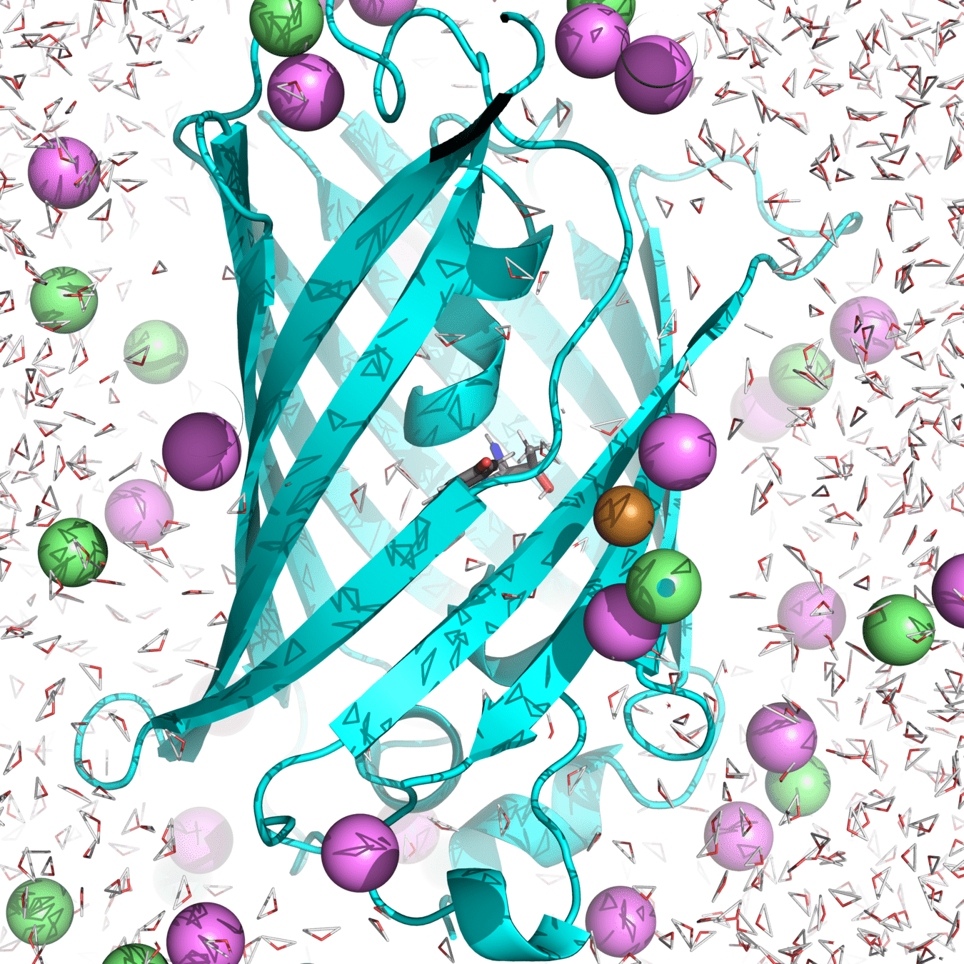
His148 stabilizes the anionic chromophore through hydrogen bonding, which influences fluorescence properties.
The hydrogen bond length fluctuates over time as atoms move between different microstates.
By sampling an ensemble of molecular simulations, we determine the mean hydrogen bond length and energy.
Our macrostate: roGFP2 in water, with 150 mM NaCl at 300 K and 1 atm
A single microstate may show a short or long bond length, but this does not represent the overall behavior.
A properly sampled ensemble gives the average bond length and the distribution of bond fluctuations.
Here is the MD trajectory
with a mean of 3.155 Å
Observing one molecular snapshot is like looking at one frame of a movie—it does not capture the full dynamics.
By simulating thousands of microstates, we capture how the hydrogen bond length varies over time.
Binding occurs when a compound/ligand interacts specifically with a protein
Protein
Ligand
Binding
Protein-
ligand
We can model this as a reversible protein-ligand binding
The change in free energy when a ligand binds to a protein
Determines binding process spontaneity
Entropy
Enthalpy
Accounts for energetic interactions
How much conformational flexibility changes
Note: Simulations capture free energy directly instead of treating enthalpy and entropy separately
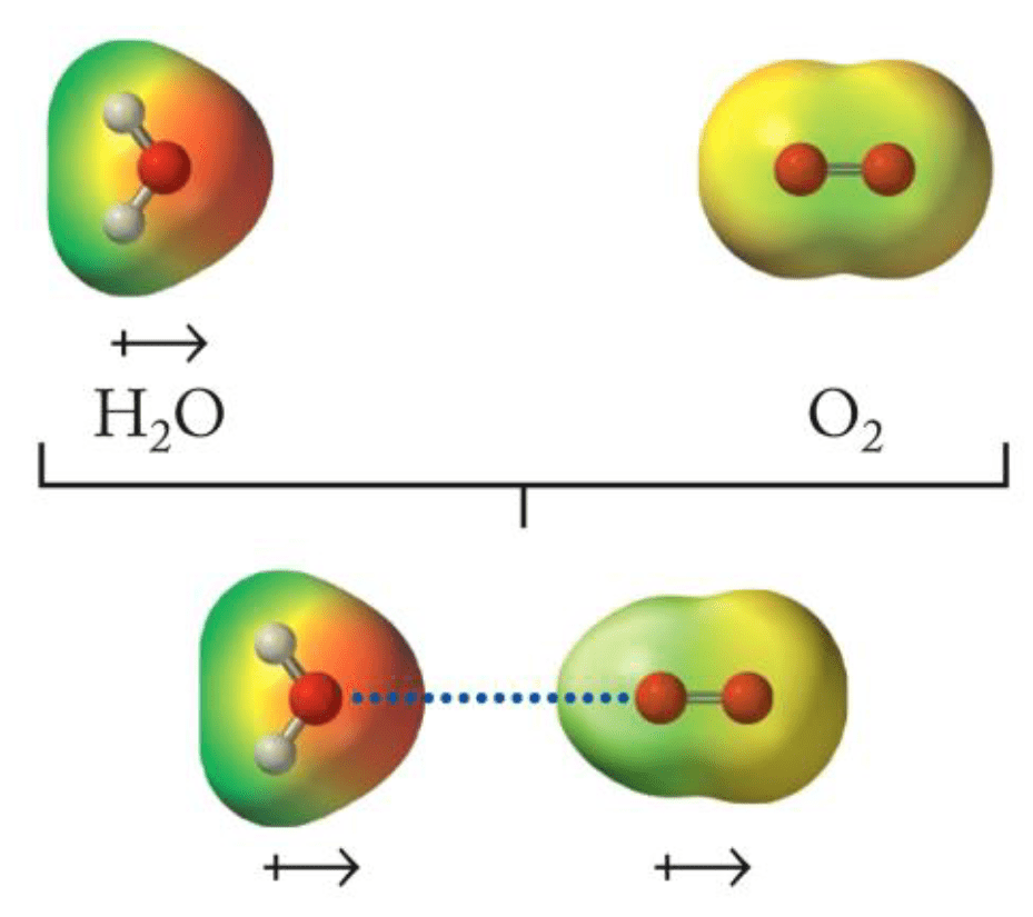
Noncovalent interactions: Electrostatics, hydrogen bonds, dipoles, π-π stacking, etc.
Ensemble differences in noncovalent interactions provide binding enthalpy
Ensemble average
(We assume no covalent bond breaking)
Our noncovalent interactions conceptual framework:
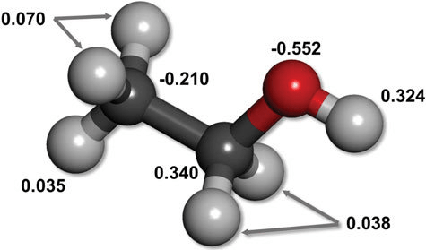
3. Regions of increased electron density are associated with higher partial negative charges
4. Electrons are mobile and can be perturbed by external interactions
1. Coulomb's law describes the interactions between charges
Molecular interactions are governed by their electron densities (Hohenberg-Kohn theorem)
This is rather difficult, so we often use conceptual frameworks to explain trends (e.g., hybridization and resonance)
2. Molecular geometry uniquely specifies an electron density
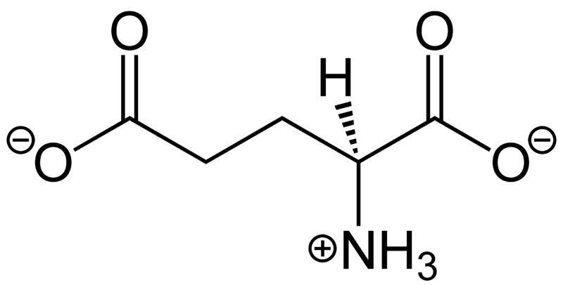
Charged molecules have a net imbalance between
This leads to net electrostatic attractions or repulsions between different atoms or molecules
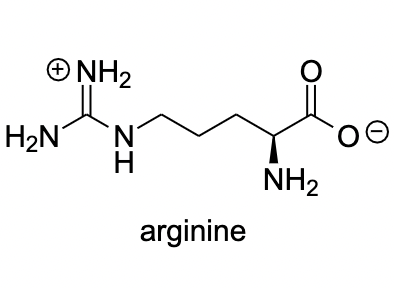
Arginine
Glycine
~5 to 20 kcal/mol per interaction
Long-Range Interaction: Can attract ligands to the binding site from a distance
Anchor Points: Often serves as key anchoring interactions in the binding site
Role in binding
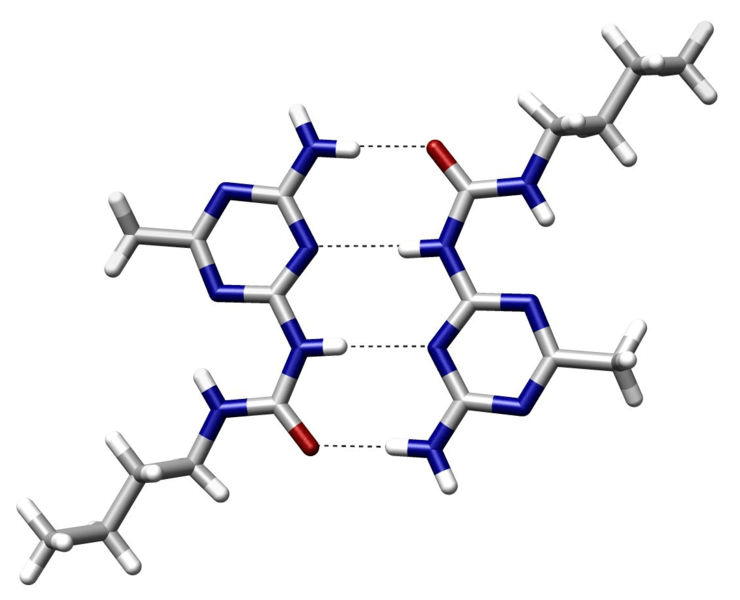
Attraction between a (donor) hydrogen atom covalently bonded to an electronegative atom and another (acceptor) electronegative atom with a lone pair
~2 to 7 kcal/mol per hydrogen bond
Strongest when the hydrogen, donor, and acceptor atoms are colinear
Specificity: Precise orientation of the ligand
Stabilization: Moderately strong interactions
Role in binding
Dynamic: Allows for adaptability of ligands
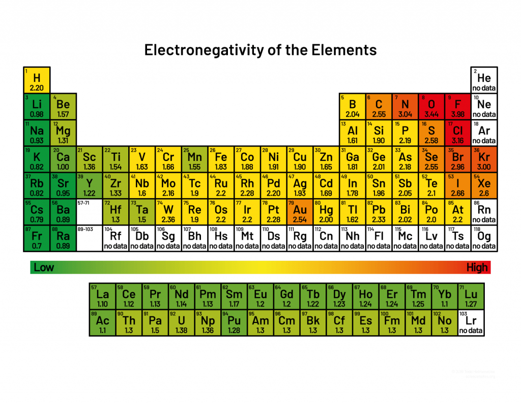
Electronegativity differences lead to unequal distribution of electron density
Unequal distribution results in regions or partial positive or partial negative charges
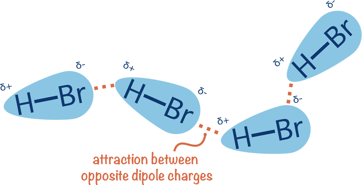
Consistent electron density spatial variation results in permanent dipoles
~0.01 to 1 kcal/mol per interaction
Directional binding: Highly directional, ensuring that the ligand aligns correctly
Flexibility: Can accommodate slight conformational changes
Role in binding
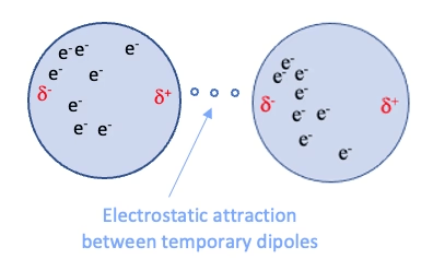
Dispersion: Electrons in molecules are constantly moving, leading to temporary uneven distributions that induce dipoles in neighboring molecules
~0.4 to 4 kcal/mol per interaction
Complementary fit: Maximizes surface contact
Flexibility: Allows small conformational changes
Role in binding
Induction: The electric field of a polar molecule distorts the electron cloud of a nonpolar molecule, creating a temporary dipole
Noncovalent interactions between aromatic rings due to overlap of π-electron clouds
~1 to 15 kcal/mol per interaction
Edge-to-face
Displaced
Face-to-face
Orientation: Proper positioning of aromatics
Selectivity: Recognition of ligands
Role in binding
One of Alex's esoteric points: "Entropy is disorder," is a massive oversimplification that breaks down in actual practice
Entropy is formally defined as
is the total number of microstates available to the system without changing the system state
Entropy is "energy dispersion"
Higher entropy implies greater microstate diversity
"System state" can be arbitrarily defined and compared as
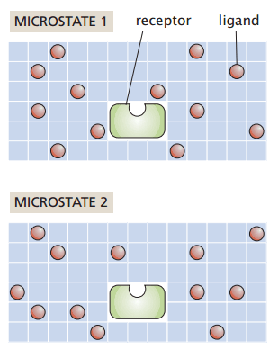
Suppose I have a system with
My macrostate (number and identity of particles, temperature, and pressure) remain constant
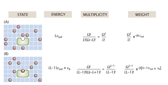
How many ways can I rearrange the ligands without binding to the receptor?
Number of ligands
Number of sites
Number of ways to choose L grid sites out of N is the binomial coefficient
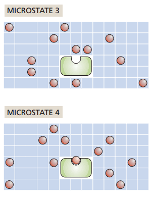
What if one ligand binds to the receptor?
How does entropy change?
Increase
No change
Decrease
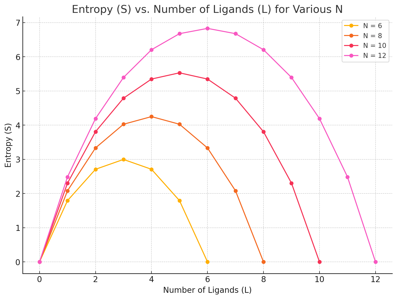
It depends on our ligand concentration!
How to interpret this: Pick a number of ligands and move to the right (L - 1), does entropy go up or down?
Lecture 10B:
Atomistic insights -
Methodology
Lecture 10A:
Atomistic insights -
Foundations
Today
Thursday
Remember: Multiple microstates (i.e., configurations) can have the same distance
We measure the ensemble probability of observing a microstate with value
Expected value of ensemble is computed by weighted mean
Note: Our denominator will always be 1 because we are not using actual partition function
2.946 Å
Note: To make our lives easier, we assume each microstate has the same energy
Energy
State
Multiplicity
Weight
The Stirling approximation
Energy
of each microstate. (In our model, this is based on number of solvated and bound ligands)
The of this system state in our macrostate ensemble
weight
Total partition function
Multiplicity
, or the the number microstates