Computing Bottom SCCs Symbolically Using Transition Guided Reduction
Nikola Beneš, Luboš Brim, Samuel Pastva, and David Šafránek


Labelled transition systems (LTS)
-
A finite set of states (S) -
A finite set of labels (L) -
A transition relation for each label:
By erasing labels, we get a normal directed graph...
Why labelled transition systems then?
SYMBOLIC COMPUTATION
Sets and relations are represented symbolically.
(We use binary decision diagrams)
With these we can build sets of forward and backward reachable states...
* saturation
LTS Operations
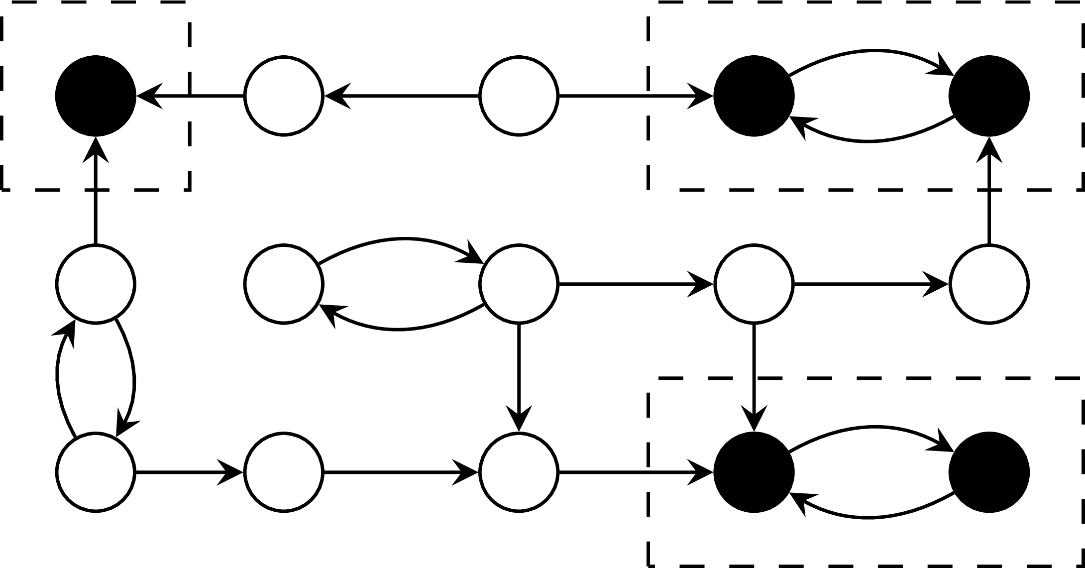
BOTTOM STRONGLY CONNECTED COMPONENTS
Goal: Identify the subsets of S that represent the bottom (terminal) strongly connected components (BSCCs).
Useful term: A subset of S is SCC-closed if whenever it contains some state x, it also contains the SCC "around" x.
"Basic" BSCC Algorithm
while S != empty:
pivot = PICK(S);
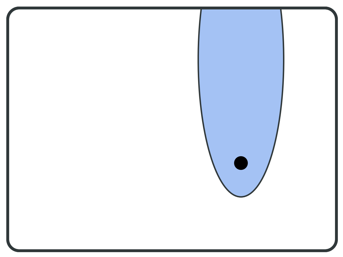
B = BWD(pivot);
F = FWD(pivot);
if F is subset of B:
report F as BSCC;
S = S \ B;
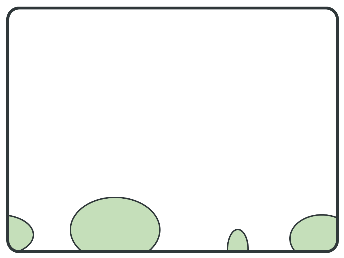
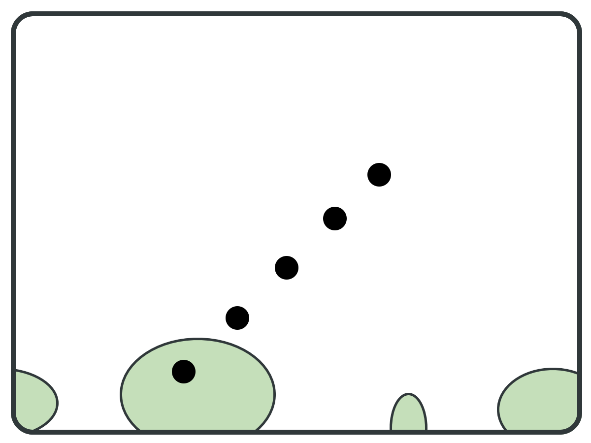
Graph

Pivot Vertex ⇒
"Basic" BSCC Algorithm
Graph
Pivot Vertex ⇒
Backward
set (B) ⇒
while S != empty:
pivot = PICK(S);
B = BWD(pivot);
F = FWD(pivot);
if F is subset of B:
report F as BSCC;
S = S \ B;
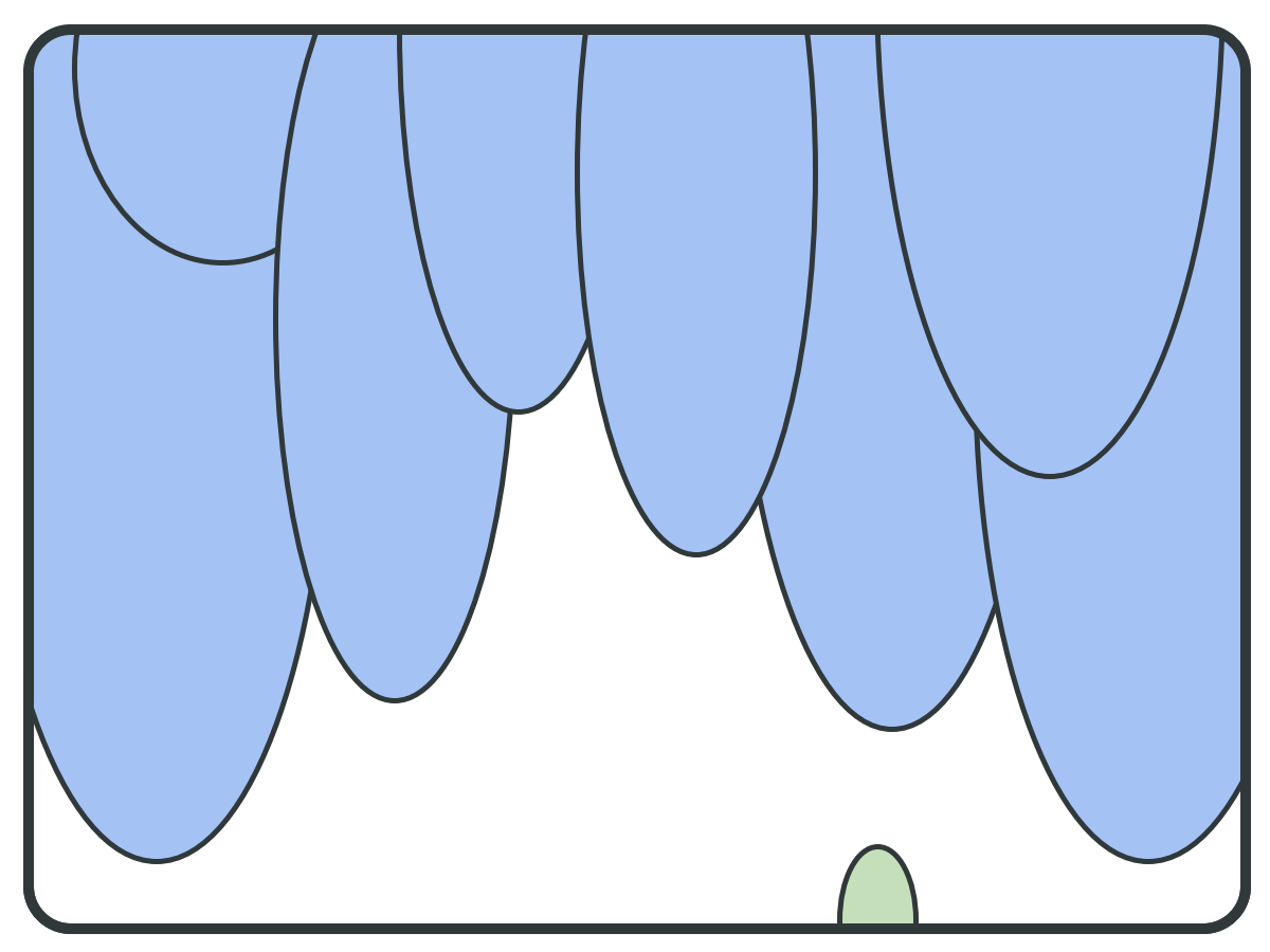
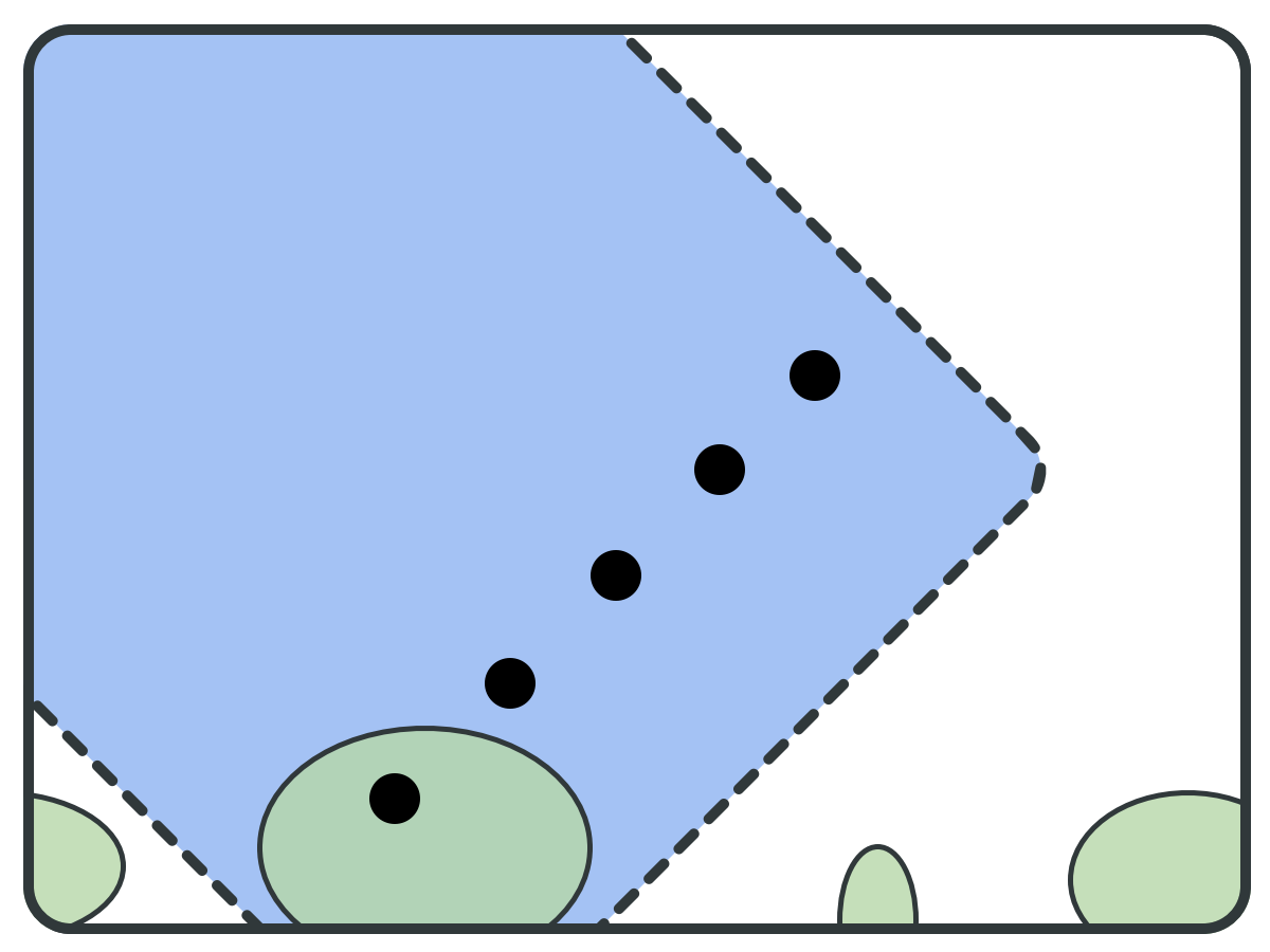
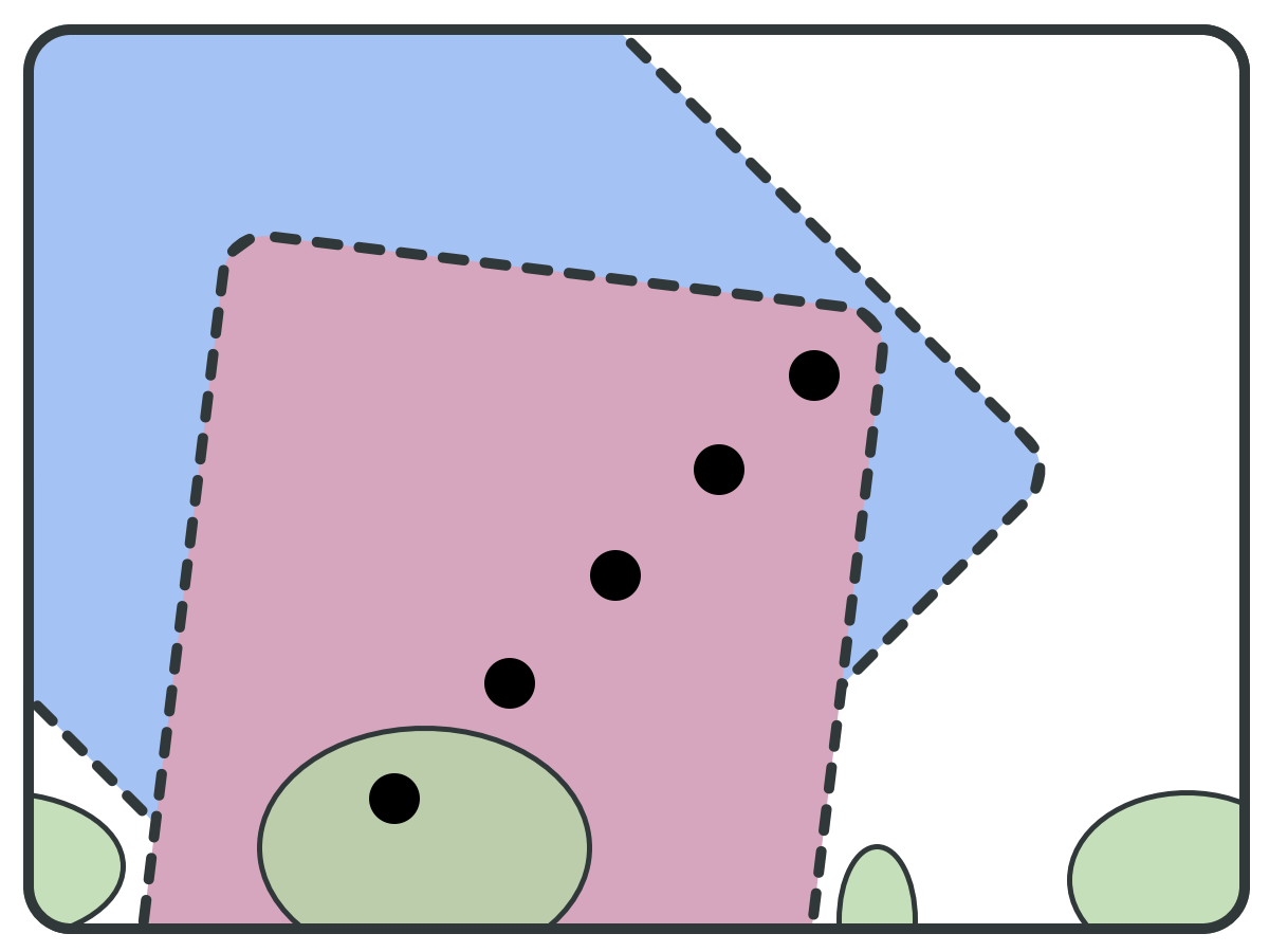
"Basic" BSCC Algorithm
Graph
Backward
set (B) ⇒
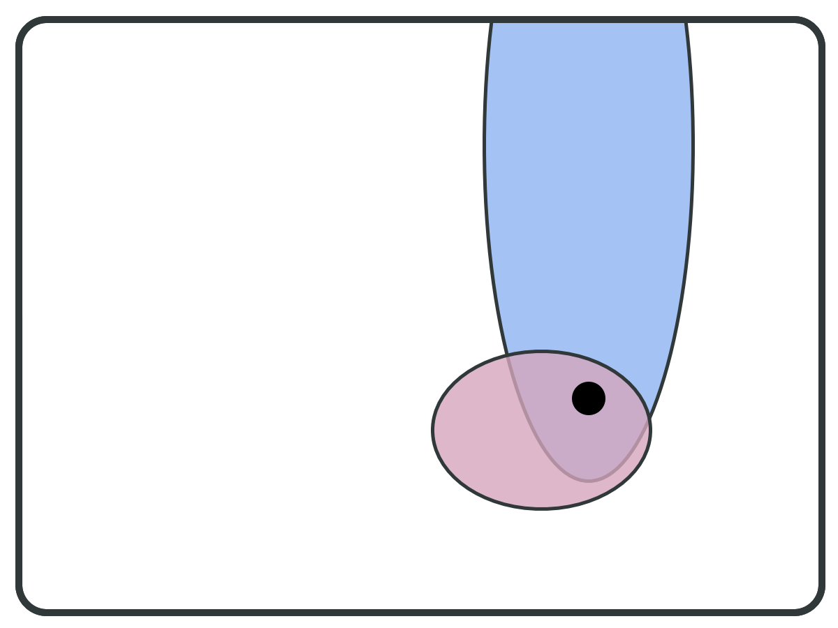
Forward
set (F) ⇒
while S != empty:
pivot = PICK(S);
B = BWD(pivot);
F = FWD(pivot);
if F is subset of B:
report F as BSCC;
S = S \ B;
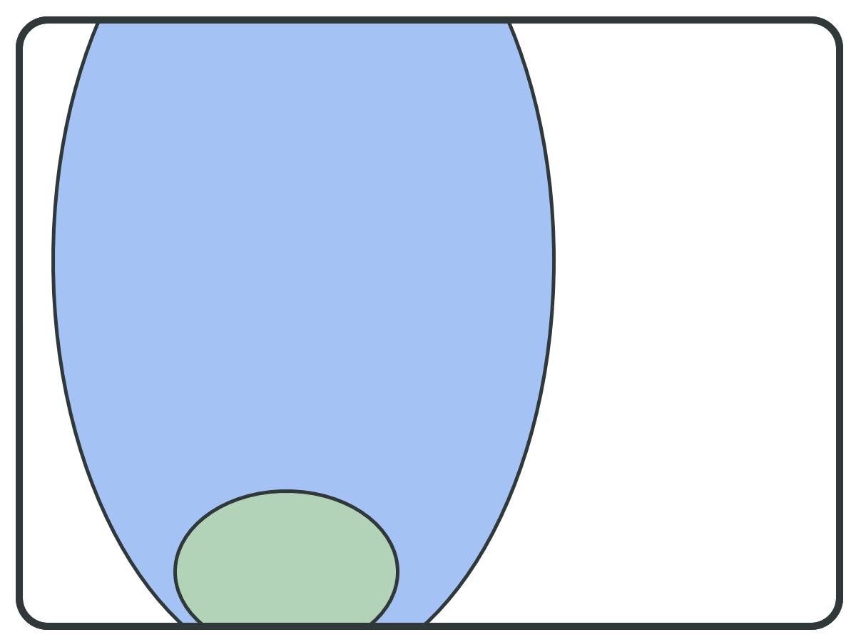
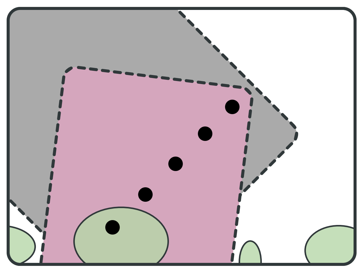
"Basic" BSCC Algorithm
Graph
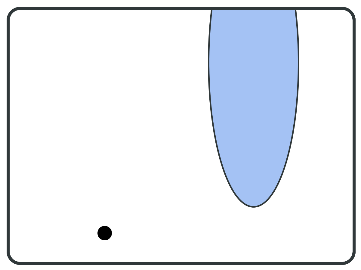
⇐ Pivot Vertex
×
Useful "tricks":
- Stop computation of F as soon as it leaves B.
- Pick pivot from F \ B when possible (instead of random)...
SCC-closed!
while S != empty:
pivot = PICK(S);
B = BWD(pivot);
F = FWD(pivot);
if F is subset of B:
report F as BSCC;
S = S \ B;
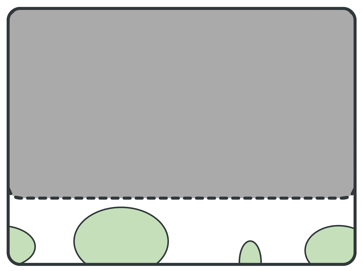
Works well when BSCC IS large, but AN interesting BSCC RARELY IS!
Graph
10^30
10^10
0.000000000000000001%
⇐
Two ways this can go wrong:
- Poor pivot selection
- Large graph diameter
×
×
×
×
×
×
×
×
y
x
x << y
Three ways...
Graph
×
reduce(S, pivots): B = BWD(pivots); F = FWD(pivots); S = S \ (B \ F); bottom = F \ B; B' = BWD(bottom); S = S \ (B' \ bottom); return S;
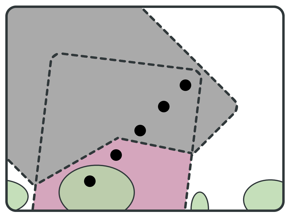
REDUCTION PRINCIPLE
⇐ Pivot Set
reduce(S, pivots): B = BWD(pivots); F = FWD(pivots); S = S \ (B \ F); bottom = F \ B; B' = BWD(bottom); S = S \ (B' \ bottom); return S;
REDUCTION PRINCIPLE
Backward set (B)
reduce(S, pivots): B = BWD(pivots); F = FWD(pivots); S = S \ (B \ F); bottom = F \ B; B' = BWD(bottom); S = S \ (B' \ bottom); return S;
REDUCTION PRINCIPLE
Backward set (B)
Forward Set
(F)
reduce(S, pivots): B = BWD(pivots); F = FWD(pivots); S = S \ (B \ F); bottom = F \ B; B' = BWD(bottom); S = S \ (B' \ bottom); return S;
REDUCTION PRINCIPLE
Backward set (B)
Forward Set
(F)
Because F is
SCC-closed
reduce(S, pivots): B = BWD(pivots); F = FWD(pivots); S = S \ (B \ F); bottom = F \ B; B' = BWD(bottom); S = S \ (B' \ bottom); return S;
REDUCTION PRINCIPLE
Backward set (B)
Forward Set
(F)
F \ B is also
SCC-closed
Who picks the pivots?
for every a in L:
  S = reduce(S, CanPost(a, S));
(T)ransition (G)uided (R)eduction
But why does it work?
All BSCCs rarely use all transition labels. Using TGR, we prune the graph based on which transitions can be actually used infinitely often in the reachable state space.
Are we done yet?
a) TGR eliminates almost all non-BSCC states. ✓
b) Performance depends on the ordering of labels.
A lot.
Interleaving?
Start reducing a.
Remove 10.000 states.
Start reducing b.
Remove 10^20 states.
...
Interleaving!
Start reducing a.
Start reducing b.
Start reducing c.
Start reducing d.
Nothing
10^20 states
5.000 states
10^6 states
The process with the smallest symbolic representation advances in every step.
- Reductions that can be computed quickly finish first.
- Completed reductions speed up the remaining processes (less remaining state space).
(I)nterleaved (T)ransition (G)uided (R)eduction
Experiments and Evaluation
125 real models, up to 2^350 states
ITGR vs. CABEAN
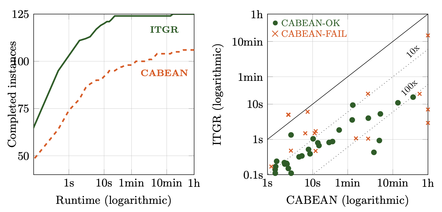
Experiments and Evaluation
125 real + 100 random, up to 2^1000 states
ITGR vs. TGR
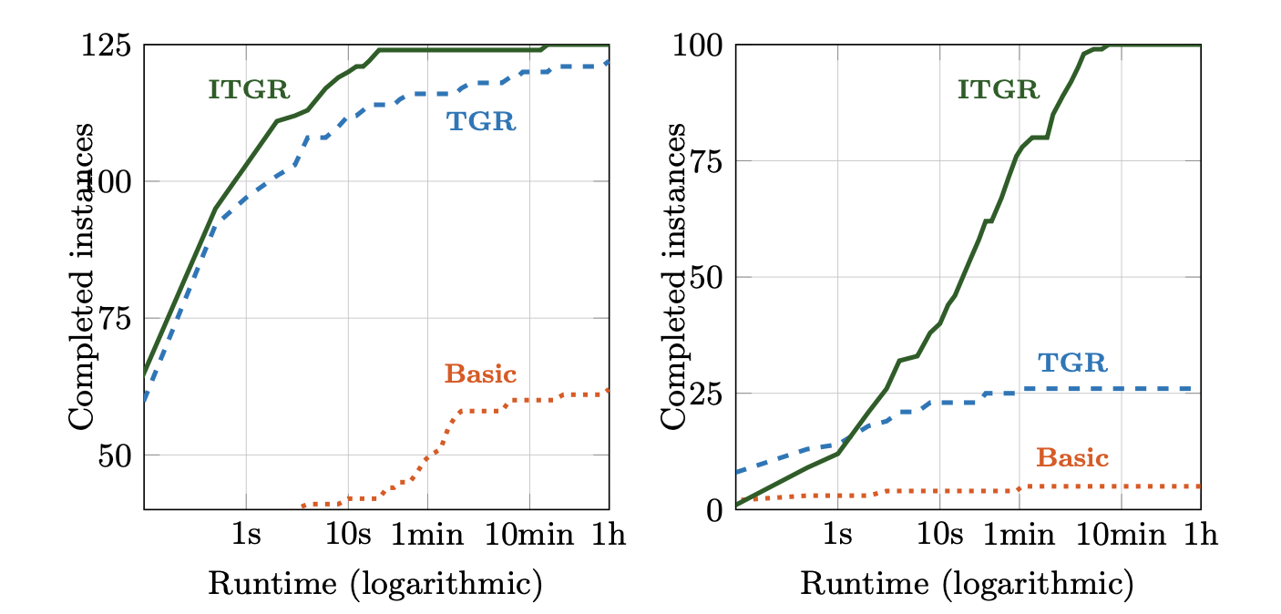
Plus another 100 models with 2^1000 only!
- General reduction principle for directed graphs.
- Transition guided reduction: Prunes states based on fireable transition labels.
- Interleaving: Improve performance and stability by performing multiple reductions simultaneously.
- Evaluation: Large real-world and generated Boolean networks.