Causal Inference for Software Traceability
int i = a \ b
assert ( i == a \ b )Requirement
Terminology
Software Traceability is the way how we follow the implementation of a requirement by establishing relations among artifacts (e.g., design documents, bug reports, code)
int i = a \ b
assert ( i == a \ b )
Requirement
Source Code
Test Cases
Most of the state-of-the-art approaches for automated traceability recovery are based on Information Retrieval
Mining concepts from code with Topic Models (Linstead et al, 2007)
Latent Dirichlet Allocation (Maskeri et al, 2008)
VSM, LDA, Jensen-Shanon, Latent Semantic Indexing and Orthogonality (Oliveto et al, 2010)
Orthogonality and Hybrid Methods (Gethers et al, 2011)
Integrating multiple source of information and TM+GA (Dit et al, 2013)
Directed Acyclic Graph (DAG) is a finite directed graph with no directed cycles

A confounder is a variable that influences both the dependent variable and independent variable causing spurious association
X (independent variable) and Y (dependent variable) are not confounded iff the following holds:
To estimate the effect of X on Y
Controlling for confounders
Gender
Recovery
Drug
Gender
Recovery
Drug
Gender
Recovery
Drug
A Counterfactual is a conditional containing an if-clause which is contrary to fact (Goodman, 1947)
If the doctor did not give the drug, then the patient was not recovered
If the doctor had not given the drug, then the patient would not have been recovered
A Counterfactual is a conditional containing an if-clause which is contrary to fact (Goodman, 1947)
If the doctor did not give the drug, then the patient was not recovered
If the doctor had not given the drug, then the patient would not have been recovered
A Counterfactual is a conditional containing an if-clause which is contrary to fact (Goodman, 1947)
If the doctor did not give the drug, then the patient was not recovered
If the doctor had not given the drug, then the patient would not have been recovered
Conditional Independence: learning the value of Y does not provide additional information about X, once we know Z
Conditional Independence: learning the value of Y does not provide additional information about X, once we know Z
The sets X and Y are said to be conditionally independent given Z if
Causal Effect vs Causal Inference
Causal Effect (in a nutshell)
Consider a dichotomous treatment A (1: LSI, 0:VSM) and a dichotomous outcome Y (1:Linked, 0:Not Linked)
Observable Outcome Variables
read Y under treatment a = 1
read Y under treatment a = 0
Causal Effect (in a nutshell)
Potential outcomes or counterfactual outcomes.
Consider this scenario for a specific Req R1 to Code C1
R1 is not Linked to C1 under LSI
R1 is Linked to C1 under VSM
Causal Effect (in a nutshell)
The treatment A has a causal effect on an individual's outcome Y if
Consider this scenario for a specific Req R1 to Code S1
Consider this powerful Research Question:
What is the average causal effect of IR baseline techniques on traceability?
In this case we need the expectation of the population
Measure of Causal Effect: Null Causal Effect
Inductive Causation (IC) Algorithm (Pearl, 1988)
- Input: p a sampled distribution on a set T of variables
- Output: some pattern (partially directed graph) compatible with p
Inductive Causation (IC) Algorithm (Pearl, 1988)
- Based on variable dependencies
- Find all pairs of variables that are dependent of each other
- Eliminate indirect dependencies
- Determine directions of dependencies
Inductive Causation (IC) Algorithm (Pearl, 1988)
X
Z
Y
Inductive Causation (IC) Algorithm (Pearl, 1988)
X
Z
Y
X
Z
Y
Inductive Causation (IC*) Algorithm (Pearl, 1988)
w
z
y
x
Inductive Causation (IC*) Algorithm (Pearl, 1988)
w
z
y
x
w
z
y
x
Inductive Causation (IC*) Algorithm (Pearl, 1988)
w
z
y
x
Inductive Causation (IC*) Algorithm (Pearl, 1988)
w
z
y
x
z
y
x
Experimental vs Observational


Software Traceability Observational or Experimental?


Automatic Repair Observational or Experimental?
Software Traceability Observational or Experimental?


Traceability Problem, the similarity values allow us to "observe" a correlation among artifacts
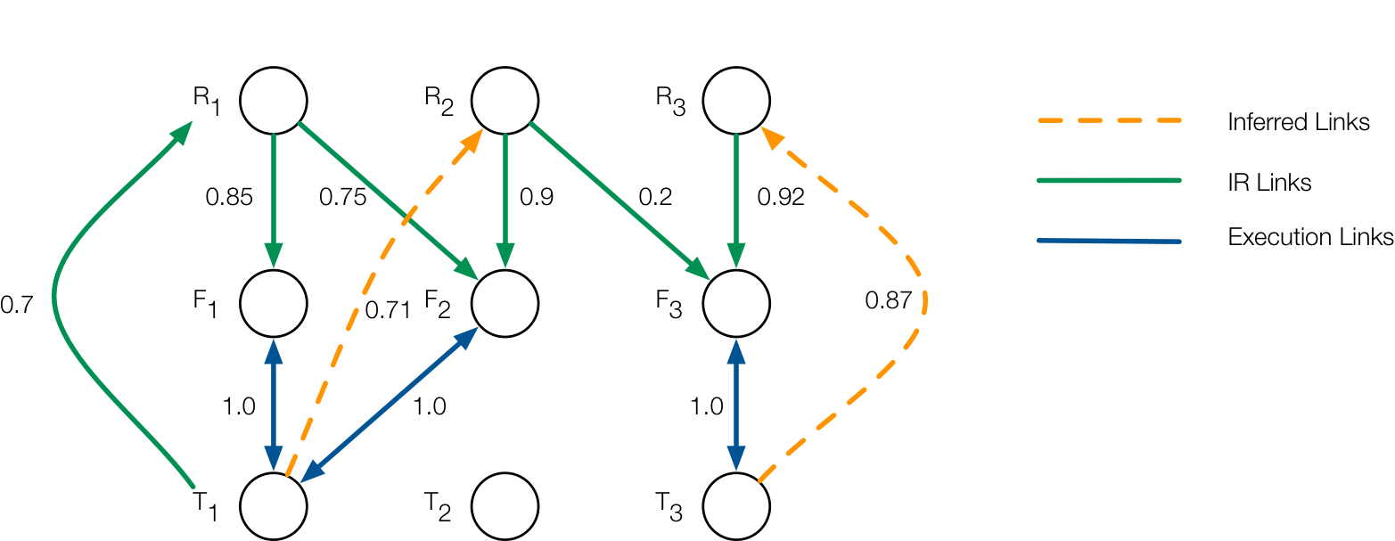
R
S
In experimental studies, we are allowed to change the individual.
To tackle the Traceability Problem by looking for correlations
Since we observe the phenomenon of traceabilty, it cannot be claimed that a Requirement Links are "Causing" Source Code Links
R
S
How can we measure the causal effect?
Randomized Experiments
From Observational to Experimental
Inductive Traceability Causation
A software traceability link is a probability distribution of an artifact respect to a set of artifacts of interest
Links
Traceability Link
A Causal Model M is composed by a set of n stochastic variables
Endogenous Variables
Exogenous Variables
For each variable T the model contains a function f such that
Set of parents
For each variable T the model contains a function f such that
Hidden causes
For each variable T the model contains a function f such that
Constant factors
The joint probability Pr({T}) can be decomposed in a Markov factorization (Pearl, 2009)
The joint probability Pr({T}) can be decomposed in a Markov factorization (Pearl, 2009)
Joint Distribution
The joint probability Pr({T}) can be decomposed in a Markov factorization (Pearl, 2009)
Conditional Independencies
Joint Distribution
A causal model M has an associated graphical representation called Causal Structure G(M)
Causal Structure of a set of variables T is a DAG in which each node corresponds to a distinct element of T, and each link represents direct functional relationship among the corresponding variables
directional separation or d-separation is the conditional independence criteria
directional separation or d-separation is the conditional independence criteria
Two nodes T and T' are d-separated by a set of C iff for every path between T,T' one of the following condition is fulfilled:
- The path contains a non-collider T_k
- The path contains a collider T_k which does not belong to C and T_k is not ancestor of an node C
A causal structure can be inferred from the set of conditional independencies present in an observed joint distribution
A causal structure can be inferred from the set of conditional independencies present in an observed joint distribution
X
Z
Y
How can we derive a probability distribution for the traceability variables?
Observational Correlation
Observational correlations
Observational correlations
Observational correlations
Correlation Vector
What do we use for categorical samples?
What do we use for categorical samples?
What do we use for categorical samples?
What do we use for categorical samples?
Generalization for multinomial
Traceability Causal Graph
Traceability Causal Graph: using interventions
Traceability Causal Graph
Case Study: LibEst
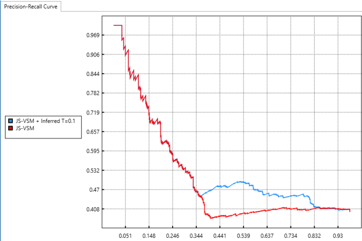
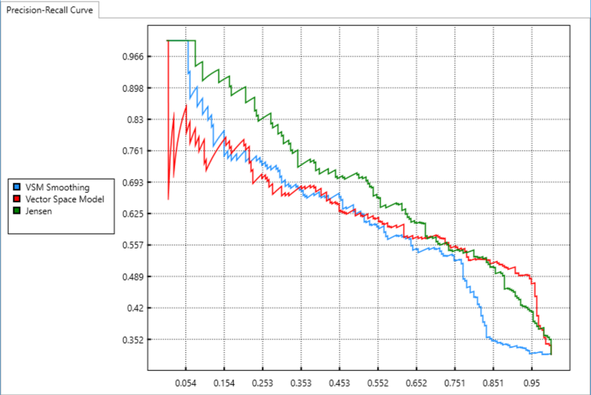
| Req File | Source File | Correlation |
|---|---|---|
| RQ11 | est_client_proxy.c | 0.0573523792522 |


| Req File | Source File | Correlation |
|---|---|---|
| RQ11 | est_client_proxy.c | 0.0573523792522 |
Finding the graph is the crux of the problem
R0
R1
R2
R5
R4
R3
[
('R0', 'R1', {'marked': False, 'arrows': ['R0']}),
('R0', 'R2', {'marked': False, 'arrows': ['R0']}),
('R1', 'R5', {'marked': False, 'arrows': []}),
('R2', 'R4', {'marked': False, 'arrows': []}),
('R3', 'R4', {'marked': False, 'arrows': []}]
R0
R1
R2
R5
R4
R3
[
('R0', 'R1', {'marked': False, 'arrows': ['R0']}),
('R0', 'R2', {'marked': False, 'arrows': ['R0']}),
('R1', 'R5', {'marked': False, 'arrows': []}),
('R2', 'R4', {'marked': False, 'arrows': []}),
('R3', 'R4', {'marked': False, 'arrows': []}]
R0
R1
R2
R5
R4
R3
[
('R0', 'R1', {'marked': False, 'arrows': ['R0']}),
('R0', 'R2', {'marked': False, 'arrows': ['R0']}),
('R1', 'R5', {'marked': False, 'arrows': []}),
('R2', 'R4', {'marked': False, 'arrows': []}),
('R3', 'R4', {'marked': False, 'arrows': []}]
R0
R1
R2
R5
R4
R3
[
('R0', 'R1', {'marked': False, 'arrows': ['R0']}),
('R0', 'R2', {'marked': False, 'arrows': ['R0']}),
('R1', 'R5', {'marked': False, 'arrows': []}),
('R2', 'R4', {'marked': False, 'arrows': []}),
('R3', 'R4', {'marked': False, 'arrows': []}]
R0
R1
R2
R5
R4
R3
[
('R0', 'R1', {'marked': False, 'arrows': ['R0']}),
('R0', 'R2', {'marked': False, 'arrows': ['R0']}),
('R1', 'R5', {'marked': False, 'arrows': []}),
('R2', 'R4', {'marked': False, 'arrows': []}),
('R3', 'R4', {'marked': False, 'arrows': []}]
R0
R1
R2
R5
R4
R3